Articolo G.A. Partial Differential Equations and Boundary Value Problems with Maple V
Подождите немного. Документ загружается.


428 Chapter 7
> u(x,y,t):=Sum(u[0,n](x,y,t),n=1..infinity)+Sum(Sum(u[m,n](x,y,t),m=1..infinity),
n=1..infinity);
u(x, y, t) :=
∞
n=1
A(0,n)cos
ω
0,n
t
+B(0,n)sin
ω
0,n
t
√
2 sin(ny)
π
+
∞
n=1
∞
m=1
2
A(m, n) cos
ω
m, n
t
+B(m, n) sin
ω
m, n
t
cos(mx) sin(ny)
π
(7.29)
> omega[m,n]:=sqrt(4*lambda[m,n]*cˆ2−gammaˆ2);
ω
m, n
:=
m
2
+n
2
(7.30)
> omega[0,n]:=subs(m=0,omega[m,n]);
ω
0,n
:=
n
2
(7.31)
We consider the special case where the initial condition functions u(x, y, 0) = f(x, y) and
u
t
(x, y, 0) = g(x, y) are given as
> f(x,y):=x*y*(Pi−y);
f(x, y) := xy(π −y) (7.32)
> g(x,y):=0;
g(x, y) := 0 (7.33)
From Section 7.5, the double Fourier coefficients A(m, n) and B(m, n) are determined from the
integrals
For m = 1, 2, 3,..., and n = 1, 2, 3,...,
> A(m,n):=eval(Int(Int(f(x,y)*X[m](x)*w(x)*Y[n](y)*w(y),x=0..a),y=0..b));A(m,n)
:=expand(value(%)):
A(m, n) :=
π
0
π
0
2xy(π −y) cos(mx) sin(ny)
π
dx dy (7.34)
> A(m,n):=factor(subs({sin(m*Pi)=0,cos(m*Pi)=(−1)ˆm,sin(n*Pi)=0,cos(n*Pi)=(−1)ˆn},
A(m,n)));
A(m, n) := −
4
−1 +(−1)
n
−1 +(−1)
m
πm
2
n
3
(7.35)

The Wave Equation in Two Spatial Dimensions 429
> B(m,n):=eval(Int(Int((f(x,y)*gamma/2+g(x,y))/(omega[m,n])*X[m](x)*Y[n](y),x=0..a),
y=0..b));B(m,n):=expand(value(%)):
B(m, n) :=
π
0
π
0
0dx dy (7.36)
> B(m,n):=simplify(subs({sin(m*Pi)=0,cos(m*Pi)=(−1)ˆm,sin(n*Pi)=0,cos(n*Pi)=(−1)ˆn},
B(m,n)));
B(m, n) := 0 (7.37)
For m = 0 and n = 1, 2, 3,...,
> A(0,n):=eval(Int(Int(f(x,y)*X[0](x)*w(x)*Y[n](y)*w(y),x=0..a),y=0..b));A(0,n):=
expand(value(%)):
A(0,n):=
π
0
π
0
xy(π −y)
√
2 sin(ny)
π
dx dy (7.38)
> A(0,n):=simplify(subs({sin(m*Pi)=0,cos(m*Pi)=(−1)ˆm,sin(n*Pi)=0,cos(n*Pi)=(−1)ˆn},
A(0,n)));
A(0,n):= −
π
√
2
−1 +(−1)
n
n
3
(7.39)
> B(0,n):=eval(Int(Int((f(x,y)*gamma/2+g(x,y))/(omega[0,n])*X[0](x)*Y[n](y),x=0..a),
y=0..b));B(0,n):=expand(value(%)):
B(0,n):=
π
0
π
0
0dx dy (7.40)
> B(0,n):=simplify(subs({sin(m*Pi)=0,cos(m*Pi)=(−1)ˆm,sin(n*Pi)=0,cos(n*Pi)=(−1)ˆn},
B(0,n)));
B(0,n):= 0 (7.41)
> T[m,n](t):=eval(T[m,n](t));
T
m, n
(t) := −
4
−1 +(−1)
n
−1 +(−1)
m
cos
m
2
+n
2
t
πm
2
n
3
(7.42)

430 Chapter 7
> T[0,n](t):=eval(T[0,n](t));
T
0,n
(t) := −
π
√
2
−1 +(−1)
n
cos
√
n
2
t
n
3
(7.43)
Generalized series terms
> u[m,n](x,y,t):=eval(T[m,n](t)*X[m](x)*Y[n](y));
u
m, n
(x,y,t):= −
8
−1 +(−1)
n
−1 +(−1)
m
cos
m
2
+n
2
t
cos(mx) sin(ny)
π
2
m
2
n
3
(7.44)
> u[0,n](x,y,t):=eval(T[0,n](t)*X[0](x)*Y[n](y));
u
0,n
(x,y,t):= −
2
−1 +(−1)
n
cos
√
n
2
t
sin(ny)
n
3
(7.45)
Series solution
> u(x,y,t):=Sum(u[0,n](x,y,t),n=1..infinity)+Sum(Sum(u[m,n](x,y,t),m=1..infinity),
n=1..infinity);
u(x, y, t) :=
∞
n=1
⎛
⎝
−
2
−1 +(−1)
n
cos
√
n
2
t
sin(ny)
n
3
⎞
⎠
+
∞
n=1
⎛
⎝
∞
m=1
⎛
⎝
−
8
−1 +(−1)
n
−1 +(−1)
m
cos
m
2
+n
2
t
cos(mx) sin(ny)
π
2
m
2
n
3
⎞
⎠
⎞
⎠
(7.46)
First few terms of sum
> u(x,y,t):=sum(u[0,n](x,y,t),n=1..1)+sum(sum(u[m,n](x,y,t),m=1..1),n=1..1):
ANIMATION
> animate3d(u(x,y,t),x=0..a,y=0..b,t=0..3,axes=framed,thickness=1);
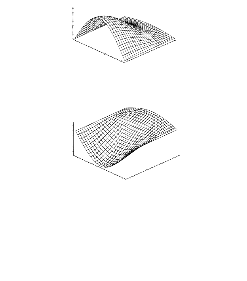
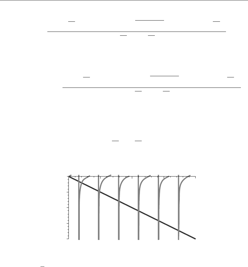
The preceding animation command illustrates the spatial-time-dependent solution for u(x, y, t).
The animation sequence in Figures 7.3 and 7.4 shows snapshots of the animation at times t = 0
and t = 2.
ANIMATION SEQUENCE
> u(x,y,0):=subs(t=0,u(x,y,t)):plot3d(u(x,y,0),x=0..a,y=0..b,axes=framed,thickness=1);

The Wave Equation in Two Spatial Dimensions 431
7
6
5
4
3
2
1
0
0
1
2
3
3
2
1
x
0.5
0.5
1.5
y
2.5
2.5
1.5
0
Figure 7.3
> u(x,y,2):=subs(t=2,u(x,y,t)):plot3d(u(x,y,2),x=0..a,y=0..b,axes=framed,thickness=1);
1
0
21
22
23
24
0
1
2
3
3
2
1
x
0.5
0.5
1.5
y
2.5
2.5
1.5
0
Figure 7.4
EXAMPLE 7.6.3: We seek the wave amplitude u(x, y, t) for the transverse wave propagation
on a thin rectangular membrane over the finite two-dimensional domain D ={(x, y) |0 <x<1,
0 <y<1}. The membrane is in a medium with no damping and the wave speed is c = 1/2.
The boundaries x = 0,x= 1, and y = 0 are held fixed, and the boundary y = 1 is constrained to
move on an elastic hinge. The initial displacement function f(x, y) and the initial speed
function g(x, y) are given as follows.
SOLUTION: The two-dimensional homogeneous wave equation is
∂
2
∂t
2
u(x, y, t) = c
2
∂
2
∂x
2
u(x, y, t) +
∂
2
∂y
2
u(x, y, t)
−γ
∂
∂t
u(x, y, t)
The boundary conditions are type 1 at x =0, type 1 at x =1, type 1 at y = 0, and type 3 at y =1:
u(0,y,t)= 0 and u(1,y,t)= 0
and
u(x, 0,t)= 0 and u(x, 1,t)+u
y
(x, 1,t)= 0

432 Chapter 7
The initial conditions are
u(x, y, 0) =
xy(1 −x)
8
and u
t
(x, y, 0) = 0
The ordinary differential equations from the method of separation of variables are
d
2
dt
2
T(t) +γ
d
dt
T(t)
+c
2
λT(t)= 0
d
2
dx
2
X(x)+αX(x)= 0
d
2
dy
2
Y(y) +βY(y)= 0
The coupling equation reads
λ = α +β
The boundary conditions on the spatial equations are
X(0) = 0 and X(1) = 0
and
Y(0) = 0 and Y(1) +Y
y
(1) = 0
Assignment of system parameters
> restart:with(plots):a:=1:b:=1:c:=1/2:unprotect(gamma):gamma:=0:
Allowed eigenvalues and corresponding orthonormal eigenfunctions are obtained from
Examples 2.5.1 and 2.5.4.
> alpha[m]:=(m*Pi/a)ˆ2;lambda[m,n]:=alpha[m]+beta[n];
α
m
:=m
2
π
2
λ
m, n
:=m
2
π
2
+β
n
(7.47)
for m = 1, 2, 3,..., and n = 1, 2, 3,..., where β
n
are the roots of the eigenvalue equation
> tan(sqrt(beta[n])*b)=−sqrt(beta[n]);
tan
β
n
=−
β
n
(7.48)
Orthonormal eigenfunctions
> X[m](x):=sqrt(2/a)*sin(m*Pi/a*x);X[r](x):=subs(m=r,X[m](x)):
X
m
(x) :=
√
2 sin(mπx) (7.49)

The Wave Equation in Two Spatial Dimensions 433
> Y[n](y):=sqrt(2)*(1/sqrt((cos(sqrt(beta[n])*b)ˆ2+b)))*sin(sqrt(beta[n])*y);Y[s](y)
:=subs(n=s,Y[n](y)):
Y
n
(y) :=
√
2 sin
√
β
n
y
cos
√
β
n
2
+1
(7.50)
Statements of orthonormality with their respective weight functions
> w(x):=1:Int(X[m](x)*X[r](x)*w(x),x=0..a)=delta(m,r);
1
0
2 sin(mπx) sin(rπx)dx = δ(m, r) (7.51)
> w(y):=1:Int(Y[n](y)*Y[s](y)*w(y),y=0..b)=delta(n,s);
1
0
2 sin
√
β
n
y
sin
√
β
s
y
cos
√
β
n
2
+1
cos
√
β
s
2
+1
dy = δ(n, s) (7.52)
Time-dependent solution
> T[m,n](t):=exp(−gamma/2*t)*(A(m,n)*cos(omega[m,n]*t)+B(m,n)*sin(omega[m,n]*t));
T
m, n
(t) := A(m, n) cos
ω
m, n
t
+B(m, n) sin
ω
m, n
t
(7.53)
Generalized series terms
> u[m,n](x,y,t):=T[m,n](t)*X[m](x)*Y[n](y);
u
m, n
(x,y,t):=
2
A(m, n) cos
ω
m, n
t
+B(m, n) sin
ω
m, n
t
sin(mπx) sin
√
β
n
y
cos
√
β
n
2
+1
(7.54)
Eigenfunction expansion
> u(x,y,t):=Sum(Sum(u[m,n](x,y,t),m=1..infinity),n=1..infinity);
u(x, y, t) :=
∞
n=1
⎛
⎜
⎝
∞
m=1
2
A(m, n) cos
ω
m, n
t
+B(m, n) sin
ω
m, n
t
sin(mπx) sin
√
β
n
y
cos
√
β
n
2
+1
⎞
⎟
⎠
(7.55)
> omega[m,n]:=sqrt(4*lambda[m,n]*cˆ2−gammaˆ2);
ω
m, n
:=
m
2
π
2
+β
n
(7.56)

434 Chapter 7
We consider the special case where the initial condition functions u(x, y, 0) = f(x, y) and
u
t
(x, y, 0) = g(x, y) are given as
> f(x,y):=x*y*(1−x)/8;
f(x, y) :=
1
8
xy(1 −x) (7.57)
> g(x,y):=0;
g(x, y) := 0 (7.58)
From Section 7.5, the double Fourier coefficients A(m, n) and B(m, n) are determined from the
integrals:
> A(m,n):=eval(Int(Int(f(x,y)*X[m](x)*w(x)*Y[n](y)*w(y),x=0..a),y=0..b));A(m,n)
:=expand(value(%)):
A(m, n) :=
1
0
1
0
1
4
xy(1 −x) sin(mπx) sin
√
β
n
y
cos
√
β
n
2
+1
dx dy (7.59)
> A(m,n):=simplify(subs({sin(sqrt(beta[n])*b)=−sqrt(beta[n])*cos(sqrt(beta[n])*b),sin(m*Pi)
=0,cos(m*Pi)=(−1)ˆm},A(m,n)));
A(m, n) :=
cos
√
β
n
−1 +(−1)
m
m
3
π
3
√
β
n
cos
√
β
n
2
+1
(7.60)
> B(m,n):=eval(Int(Int((f(x,y)*gamma/2+g(x,y))/(omega[m,n])*X[m](x)*Y[n](y),x=0..a),
y=0..b));B(m,n):=expand(value(%)):
B(m, n) :=
1
0
1
0
0dx dy (7.61)
> B(m,n):=simplify(subs({sin(sqrt(beta[n])*b)=−sqrt(beta[n])*cos(sqrt(beta[n])*b),sin(m*Pi)
=0,cos(m*Pi)=(−1)ˆm},B(m,n)));
B(m, n) := 0 (7.62)
> T[m,n](t):=eval(T[m,n](t));
T
m, n
(t) :=
cos
√
β
n
−1 +(−1)
m
cos
m
2
π
2
+β
n
t
m
3
π
3
√
β
n
cos
√
β
n
2
+1
(7.63)
Generalized series terms

The Wave Equation in Two Spatial Dimensions 435
> u[m,n](x,y,t):=eval(T[m,n](t)*X[m](x)*Y[n](y));
u
m, n
(x,y,t):=
2 cos
√
β
n
−1 +(−1)
m
cos
m
2
π
2
+β
n
t
sin(mπx) sin
√
β
n
y
m
3
π
3
√
β
n
cos
√
β
n
2
+1
(7.64)
Series solution
> u(x,y,t):=Sum(Sum(u[m,n](x,y,t),m=1..infinity),n=1..infinity);
u(x, y, t) :=
∞
n=1
⎛
⎝
∞
m=1
2 cos
√
β
n
−1 +(−1)
m
cos
m
2
π
2
+β
n
t
sin(mπx) sin
√
β
n
y
m
3
π
3
√
β
n
cos
√
β
n
2
+1
⎞
⎠
(7.65)
Evaluation of the eigenvalues β
n
from the roots of the eigenvalue equation yields
> tan(sqrt(beta[n])*b)+sqrt(beta[n])=0;
tan
β
n
+
β
n
= 0 (7.66)
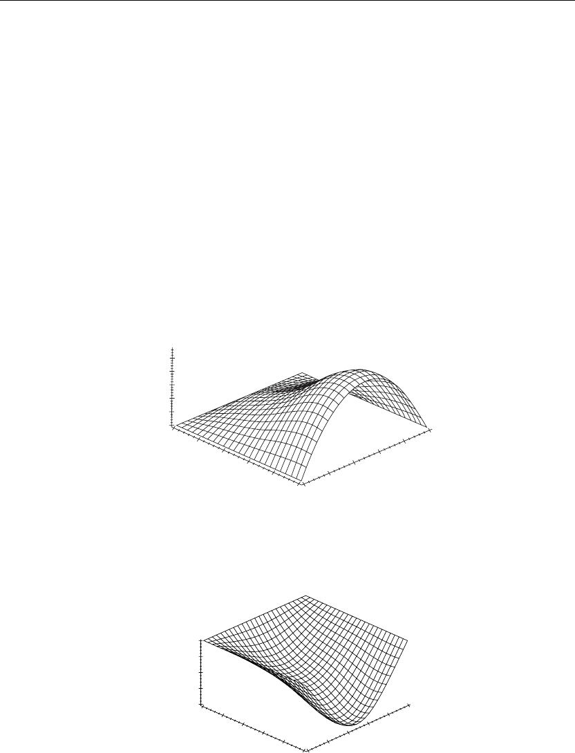
> plot({tan(v),−v},v=0..20,y=−20..0,thickness=10);
v
5101520
y
220
215
210
25
0
Figure 7.5
If we set v =
√
βb, then the eigenvalues β
n
are found from the intersection points of the curves
shown in Figure 7.5. Some of these eigenvalues using the Maple fsolve command are
evaluated here:
> beta[1]:=(1/bˆ2)*(fsolve((tan(v)+v),v=1..3))ˆ2;
β
1
:= 4.115858365 (7.67)
> beta[2]:=(1/bˆ2)*(fsolve((tan(v)+v),v=3..6))ˆ2;
β
2
:= 24.13934203 (7.68)

436 Chapter 7
> beta[3]:=(1/bˆ2)*(fsolve((tan(v)+v),v=6..9))ˆ2;
β
3
:= 63.65910654 (7.69)
First few terms of sum
> u(x,y,t):=eval(sum(sum(u[m,n](x,y,t),m=1..3),n=1..3)):
ANIMATION
> animate3d(u(x,y,t),x=0..a,y=0..b,t=0..3,axes=framed,thickness=1);
The preceding animation command illustrates the spatial-time-dependent solution for u(x, y, t).
The animation sequence in Figures 7.6 and 7.7 shows snapshots of the animation at the two
times t = 0 and t = 4.
ANIMATION SEQUENCE
> u(x,y,0):=subs(t=0,u(x,y,t)):plot3d(u(x,y,0),x=0..a,y=0..b,axes=framed,thickness=1);
0.025
0.02
0.015
0.01
0.005
0
0
0.2
0.4
0.6
0.8
1
1
0.8
0.6
0.4
x
y
0.2
0
Figure 7.6
> u(x,y,4):=subs(t=4,u(x,y,t)):plot3d(u(x,y,4),x=0..a,y=0..b,axes=framed,thickness=1);
20.005
20.01
20.02
20.015
0
0
0.2
0.4
y
0.6
0.8
11
0.8
0.6
0.4
x
0.2
0
Figure 7.7

The Wave Equation in Two Spatial Dimensions 437
7.7 Wave Equation in the Cylindrical Coordinate System
If we replace the Laplacian operator from Section 7.2 in rectangular coordinates in two
dimensions to its equivalent in cylindrical coordinates, then the nonhomogeneous partial
differential equation for wave phenomena in the cylindrical coordinate system in two
dimensions is given as
∂
2
∂t
2
u(r,θ,t)= c
2
⎛
⎝
∂
∂r
u
(
r, θ, t
)
+r
∂
2
∂r
2
u(r,θ,t)
r
+
∂
2
∂θ
2
u(r,θ,t)
r
2
⎞
⎠
−γ
∂
∂t
u(r,θ,t)
+h(r,θ,t)
where r is the coordinate radius of the system and θ is the polar angle. The γ term takes into
account any viscous damping in the medium, and h(r,θ,t)takes into account any external
applied forces acting on the system. There is no z dependence here because we will only
examine wave phenomena along very thin membranes or plates that have no extension along
the z-axis.
As for the rectangular coordinate system, we can write the preceding equation in terms of the
linear operator for the wave equation in cylindrical coordinates as
L(u) = h(r,θ,t)
where the wave operator in cylindrical coordinates reads
L(u) =
∂
2
∂t
2
u(r,θ,t)−c
2
⎛
⎝
∂
∂r
u(r,θ,t)+r
∂
2
∂r
2
u(r,θ,t)
r
+
∂
2
∂θ
2
u(r,θ,t)
r
2
⎞
⎠
+γ
∂
∂t
u(r,θ,t)
Generally, one seeks a solution to this equation over the finite two-dimensional domain
D ={(r, θ) |0 <r<a,0 <θ<b} subject to the following homogeneous boundary conditions:
|
u(0,θ,t)
|
< ∞
κ
1
u(a, θ, t) +κ
2
u
r
(a,θ,t)= 0
κ
3
u(r, 0,t)+κ
4
u
θ
(r, 0,t)= 0
κ
5
u(r,b,t)+κ
6
u
θ
(r,b,t)= 0
along with the two initial conditions
u(r, θ, 0) = f(r, θ) and u
t
(r, θ, 0) = g(r, θ)
We now attempt to solve the homogeneous version [no external applied forces, h(r,θ,t)= 0] of
this partial differential equation using the method of separation of variables. We set
u(r,θ,t)= R(r)(θ)T(t)
