Armstrong M., et al. Plurigaussian simulations in geosciences

Подождите немного. Документ загружается.

As E[1

Iru

¼P

½I  ru

h(u,v)dv = k

ﬃﬃﬃﬃﬃﬃ

exp

u



 P

ðI  ruÞ

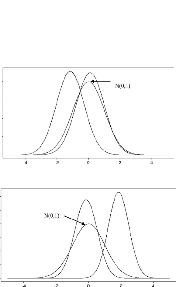
Thisshows that the marginal densityof Z(x) given that Z(y) 2 I, is no longer

gaussian. It is proportional to a gaussian density but is multiplied by the probability

that the ﬁrst variable lies in the interval, I  ru. To illustrate the impact of this

change, we have plotted this distribution for two intervals: [0.5, 0.5] and [2, 3],

and for two different correlation factors, 0.5 and 0.8. Figures 7.1 and 7.2 present

the resulting curves.

Fig. 7.1 Probability densities functions for the marginal distributions for the two intervals, for the

case where r ¼0:5 together with the N(0,1) density for comparison purposes

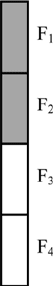
Fig. 7.2 Probability densities functions for the marginal distributions for the two intervals, for the

case where r ¼ 0:8 together with the N(0,1) density for comparison purposes

110 7 Gibbs Sampler

Simulating Z(x) and Z(y) When Both Belong to Intervals

Now suppose that Y(x) belongs to I

and Y(y) belongs to I

. Th eir joint density is

h(u,v) ¼ kg(u,v)1

ðuÞ1

ðvÞ

where k is the appropriate normation factor.

h(u,v) =

ﬃﬃﬃﬃﬃﬃ

exp 

ðu  rv



ðuÞ

ﬃﬃﬃﬃﬃﬃ

exp 



ðvÞ

As expected, the marginal distributions are no longer gaussian or even truncated

gaussian. Integrating with respect to u gives

h(u,v)du /

ﬃﬃﬃﬃﬃﬃ

ðI

 rvÞ exp

v



ðvÞ (7.3)

Similarly integrating with resp ect to v gives

h(u,v)dv /

ﬃﬃﬃﬃﬃﬃ

ðI

 ruÞ exp

u



ðuÞ (7.4)

Because of the increasing difﬁcult in simulating these distributions directly as the

number of interval constraints increases, we rapidly reach the point where direct

simulation is no longer practicable and we have to resort to an indirect approach

such as the Gibbs sampler.

These examples suggest the idea of using a two step procedure to conditionally

simulate gaussian values when some of them are constrained to lie in speciﬁed

intervals. The two steps are:

1. Generating gaussian values at data points, in the prescribed intervals and with

the right covariance structure

2. Using any algorithm for conditionally simulating gaussian random functions

given the values generated in step (1)

Direct Simulation Using an Acceptance/Rejection Procedure

Having seen that the ﬁrst stepis to generatea set of gaussian valuesat samplepoints,

the next question is how this should be done. We might be tempted to try an

acceptance/rejection procedure, by generating gaussian values with the right covari-

ance structure and rejecting those lying outside the speciﬁed intervals. If only 10 or

20 samples were available this could be done directly using an LU decomposition

Simulating Z(x) and Z(y) When Both Belong to Intervals 111

(i.e. a Cholesky decomposition of the covariance matrix). The LU decomposition

could be carried out for much larger matrices (up to about 500  500). The limiting

factor in the procedureis the rate of rejection.For example, suppose that ten samples

wereavailableandthattherewereonlytwofacieseachpresent50%ofthetime.Then

if there was no spatial correlation (pure nugget effect), the probability of getting all

ten values in the right intervals would be 1 in 2

; that is, about 1 in 1,000. This

procedure becomes prohibitively slow as the number of samples increases. As there

are usually hundreds or thousands of data in mining and petroleum applications,

another approach is needed. This is why we have to resort to more complicated

methods.

Gibbs Sampler

Statisticians routinely use iterative methods based on Markov chain Monte Carlo

simulations (MCMC, for short) for sampling complicated distributions and for

estimating parameter values. The best known are the Hastings-Metropolis algo-

rithm and the Gibbs sampler. The latter is a particular case of the Hastings-

Metropolis method. See Meyn and Tweedie (1993), Cowles and Carlin (1996)

and Robert (1996) for information on these methods. Freulon (1992) and Freulon

and de Fouquet (1993) adapted the Gibbs sampler to truncated gaussian simula-

tions. To introduce this technique, we present an example to show how this method

works and to illustrate the concept of convergence.

Four Sample Example

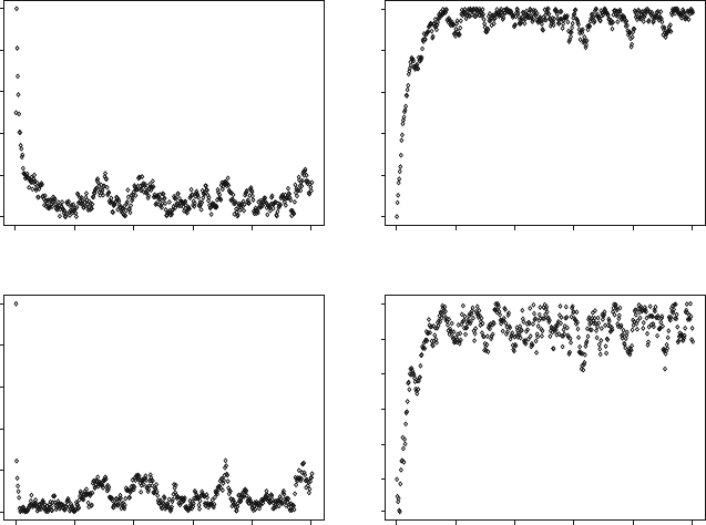
Suppose that there are only two lithotypes F

and F

, and that they are present in

equal proportions. So it is natural to use a zero threshold to separate them. Negative

Fig. 7.3 Simpliﬁed well or drill hole containing four samples

112 7 Gibbs Sampler

gaussian values correspond to F

; positive ones, to F

.Figure 7.3 shows a simpliﬁed

well or drill hole containing four samples, with the top two belonging to F

and the

other two belonging to F

. The gaussian values assigned to the top samples must be

negative, the others have to be positive.

The procedure relies on the standard decomposition of the gaussian random

function into its simple kriging estimate and an orthogonal residual.

Z(xÞ¼Z

(xÞþs

R(x)

where the index SK denot es the simple kriging estimate or its variance and R(x) is a

N(0,1) residual.Note thatfor gaussian random variables, the SK estimate equals the

conditional expectation.

Exponential Variogram

Suppose that the four samples are 1m apart and that the underlying variogram for

the gaussian s is an exponential with a unit sill and a scale parameter a ¼ 2 m (i.e. a

practical range of 6 m). The SK weights for estimating the top point using the other

three points as data are:

¼ 0: 61; l

¼ 0; l

¼ 0 and s

¼ 0:63 ) s

¼ 0:79

(Points are numbere d from the top down). By symmetry the weights are the same

but in the reverse order when kriging the fourth point from the other three. The

weights for the second point (or similarly the third one) are:

¼ 0: 44; l

¼ 0:44; l

¼ 0 and s

¼ 0: 46 ) s

¼ 0:68

As the conﬁguration does not change from one iteration to the next the weights

remain the same.

Step 1: Initialising the Procedure

The ﬁrst step consists of choosing gaussian values that belong to the appropriate

intervals. Here we select (1, 1, þ1, þ1)

Step 2: Iterative Procedure

Simple kriging is applied to the points in turn. For example, the value of the top

point is kriged using the other three points as input data. Then we move down to the

second p oint and krige it using the initial values for the points below it and the new

Gibbs Sampler 113

updated value for the top point. After completing the second point we move down

to the third one which is kriged using the updated values for the points above it and

the old value for the point below it. Similarly for the fourth point. When all the

points have been updated by kriging , one iteration has been completed.

Point No 1

The kriged estimate for Z(x

), abbreviated to Z(1), based on the initial values (i.e.

1, +1, +1) for the other three points is:

ð1Þ¼1  0 :61 þ 1 0 þ 1  0 ¼0:61

And the correspond ing residual must satisfy

R(1) ð0:61Þ=0:79 ¼ 0:77

Suppose for argument’s sake that we draw a value of 0.52 (from a N(0,1) distribu-

tion). Then the updated value would be

Zð1Þ¼0:61 þ 0:79  0:52 ¼0:20

Point No 2

The kriged estimate for Z(2) based on the initial values for Z(3) and Z(4), and the

updated value of Z(1) is:

ð2Þ¼0:20  0 :44 þ 1 0:44 þ 1  0 ¼ 0:42

The corresponding residual must satisfy

Rð2Þ0:42=0:68 ¼ 0:62

If we draw a value of 0.75, then the updated value of Z(2) is

Zð2Þ¼0:42 þ 0:68 0:75 ¼0:09

Point No 3

Following the same procedure, the kriged estimate for Z(3) and the inequality to be

satisﬁed by its residual are

ð3Þ¼0:20  0  0:09  0:44 þ 1  0:44 ¼þ0:40

114 7 Gibbs Sampler

R(3)  0:40=0:68 ¼ 0:59

If we draw a value of 0.28, then the updated value of Z(3) is 0.21.

Point No 4

In the same way, the kriged estimate for Z(4) and the inequality to be satisﬁed by its

residual are

ð4Þ¼0 ð0:20Þþ0 ð0:09Þþ0: 61  0:21 ¼ 0:13

R(4) 0:13=0:79 ¼0:16

Drawing a value of 0.63 would give an updated value of 0.63 for Z(4).

Results

Table 7.1 summarises the intermediate results during ﬁrst iteration. This updating

procedure is repeated iteratively, in general for several hundred or several thousand

iterations. Table 7.2 shows the results of the ﬁrst ﬁve iterations.

Alternative Updating Strategies

In the previous example, individual points were sequentially updated. A variant of

this consists of sequentially updating from the top down, then from the bottom up

on the next iteration.

Table 7.1 Successive steps in the ﬁrst iteration of this Gibbs sampler

Table 7.2 Results of ﬁrst ﬁve iterations of the Gibbs sampler

Pt N



Initial No 1 No2 No3 N



1 1 0.20 0.37 1.34 0.34 0.13

2 1 0.09 0.35 0.24 0.31 0.20

3 þ1 þ0.21 þ0.15 þ0.05 þ0.19 þ0.20

4 1 þ0.63 þ0.86 þ0.10 þ0.26 þ0.32

Gibbs Sampler 115

Blocking Factor

It is also possible to update blocks of points simultaneously. For example, the four

points could be grouped into two blocks each consisting of two points. There are

three possible groupings of this type:

Points 1 & 2 and Points 3 & 4

Points 1 & 3 and Points 2 & 4

Points 1 & 4 and Points 2 & 3

In the ﬁrst case, the values of the top two points are updated using the values of

the other two as the conditioning data (i.e. using kriging) and simulated in the right

interval with the right correlations, and vice versa for the other pair. We will

illustrate this procedure later in the chapter. As was shown in Chap. 2 suitably

chosen blocking strategies can signiﬁcantly improve the speed of convergence.

Experimentally Testing Convergence

Having seen how the procedure works, several questions need to be answered.

Firstly, does the algorithm converge? If so, after how many iterations? What factors

affect the speed of convergence? How should we choose the initial values?

Burn-in Period

In this section we illustrate the difference between the initial burn-in period and the

subsequent stationary part of the Markov chain. To do this we continue the previous

examplebutthevariogramischangedtoa gaussianmodelwitha practicalrangeof3.

So the correlation between adjoining samples is 0.95. Five hundred iterations of the

corresponding Gibbs sampler were run starting from a very extreme set of initial

values (+5,+5,5,5). This choice lengthens the initial burn-in period, making it

visually much more obvious.

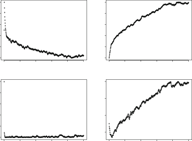
Figure 7.4 shows the output for each component as a function of the number of

iterations. The values of the ﬁrst component (top left) decrease steadily from the

initial value of þ5 until they are below 1.0. The curve seems to stabilise after

approximately 100 iterations so the burn-in period must be at least this long.

Similarly for the third and fourth components. But it appears to be much shorter

for the other component (bottom left), about 20 iterations. This shows that the burn-

in period need not be the same for all components in a Gibbs sampler. In MCMC

theory it is well-known that different states can have different rates of convergence;

see Meyn and Tweedie (1993, pp 362–363).

The implications of not necessarily having the same burn-in period for all

components are important in practice. When there are only four components it is

116 7 Gibbs Sampler

possible to check the convergence of all of them but if there were 1,000 samples it

would be virtually impossible to inspect the output of the Gibbs sampler for all

1,000 components. We could only check a few of them visually and we might have

the bad luck to choose those with shorter burn-ins. Inspecting the results for

selected components gives us an idea of the burn-in period but it is not foolproof.

Effect of the Range on the Burn-in Period

Several factors including the range of the variogram and the number of components

havea markedeffecton the length of the burn-in period.To illustrate the effectofthe

range, we repeated the previous example using a practical range of 5 instead of 3.

Thisincreasesthecorrelationbetweenadjoiningsamplesfrom0.95to0.98.Figure7.5

shows the output.

Whereas the burn-in period for the ﬁrst component was about 100 beforehand,

it is now closer to 500. Conversely decreasing the range would decrease the

burn-in period. Looking at Fig. 7.5 we also notice how smooth the curves are

0 100 200 300 400 500

0246810

–5 –4 –3 –2 –1 0

012345

–6 –5 –4 –3 –2 –1 0

Fig. 7.4 Output of the Gibbs sampler for all 4 components for 500 iterations, starting from initial

values of (þ5,þ5,5,5). The second component (lower left) seems to stabilise after about 20

iterations components whereas the other three are much slower. They take at least 100 iterations to

reach their stationary distribution

Experimentally Testing Convergence 117

compared to the corresponding ones in Fig. 7.4. The strong serial correlation

between successive values makes it more difﬁcult to determ ine whether the Markov

chain has converged.

These two examples show that it is not simple to judge whether a Gibbs sampler

has reached its stationary distribution just by studying the output from a single run

(even a very long one). It would be better to run a large number of samplers in

parallel and study their output after 1, 5, 10, ..., 50 iterations and so on. Ideally we

should compare the experimental distribution of the output with the stationary

distribution. How could this be tested experimentally?

A multivariate normal distribution is fully speciﬁed when the means and the

covariance matrix are known. By extension, a truncated gaussian is fully deﬁned

whenthetruncationthresholdsareknowntogetherwiththemeansandthecovariance

matrix for the full distribution. Having said that, it is clear that after truncation the

means are not going to be the same as before. See (7.3) and (7.4). Nor are the vari-

ances or the correlations. In the case under study, the four components come from

a quadrivariate normal distribution with the covariance matrix given in Table 7.3.

Because of the high correlation between adjoining samples, its density is an

elongated cigar shape. Figure 7.6 shows a diagram representing the bivariate

densities of X

and X

, and X

and X

respectively. The impact of different types

0 100 200 300 400 500 0 100 200 300 400 500

810

012345

–5 –4 –3 –2 –1 0–6 –4 –2 0

Fig. 7.5 Output of the Gibbs sampler for the ﬁrst of 4 components for 500 iterations, starting from

initial values of (þ5,þ5,5,5). Compared to Fig. 7.4, the correlation between adjoining points

has been increased from 0.95 to 0.98. Note the increase in the burn-in period

118 7 Gibbs Sampler

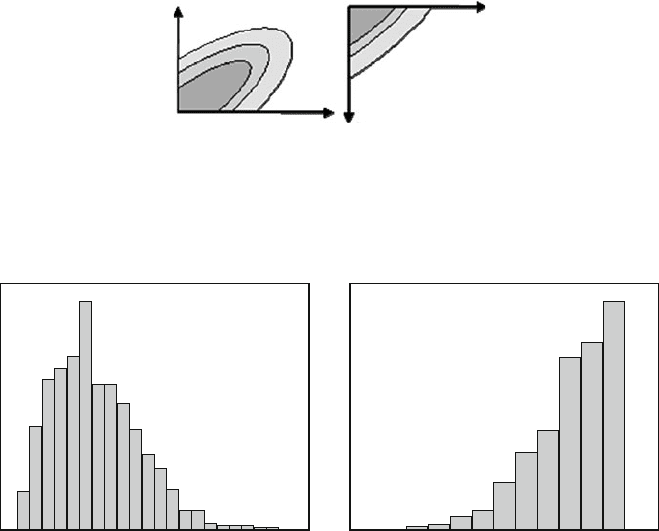
of truncations is evident from these. In one case, we are dealing with the elongated

part of the ellipse whereas in the other, it is merely a triangular “corner”. Intuition

can often be misleading when trying to guess the properties of truncated gaussian

distributions. For example many people expect the marginal distributions in this

example to be “half gaussians”. The marginal distributions given in Fig. 7.7 show

just how wrong intuition can be and also conﬁrms what was shown in the two

variable case given at the beginning of the chapter.

The Impact of Different Parallel Runs

Up till now we have illustrated the difference between the burn-in period and the

stationary part by focussing on individual components. An alternative is to run

Table 7.3 Quadrivariate

covariance matrix for

the 4-sample case

10:95 0:80 0:61

0:95 1 0:95 0:80

0:80 0:95 1 0:95

0:61 0:80 0:95 1

Fig. 7.6 Schematic representation of the bivariate densities of X

and X

(left) and of X

and

(right)

Fig. 7.7 The marginal distributions of X

and of X

Experimentally Testing Convergence 119