Armstrong M., et al. Plurigaussian simulations in geosciences

Подождите немного. Документ загружается.

on the gaussian coordinate axes. The end points of these projections can be

considered as thresholds. Each rectangular box is deﬁned by 2

thresholds (some

of them can be inﬁnite). When we know 2

 1 of them, it is possible to invert the

equation

xðÞ¼

;...;z

ðÞdz

...dz

numerically to ﬁnd the last unknownthreshold. Ifwe have N gaussian functions and

M facies, we have M  2

thresholds. As we do not allow “empty space”, our

rectangular boxes constitute a partition of this space. This considerably decreases

the number of independent thresholds. For example, if we include the inﬁnite

thresholds, we have:

M þ 1 thresholds with 1 gaussian function (i. e., truncated gaussian method)

M þ 3 thresholds with 2 gaussian functions

M þ 5 thresholds with 3 gaussian functions

M þ 2N1 thresholds with N gaussian functions

which means M1 ﬁnite independent thresholds.

Choice of the Partition

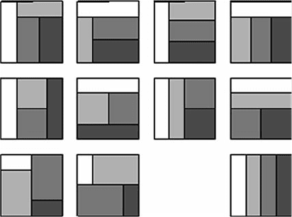
Even after having decided to use a rectangular partition, there are many possible

layouts. For example with two gaussian functions and four lithofacies, we have ten

possibilities, plus one which is equivalent to the case with only one gaussian

function. Figure 5.7 shows these partitions. With 6 facies, we have approximately

140 possibilities. This shows that we will not be able to test all the possible

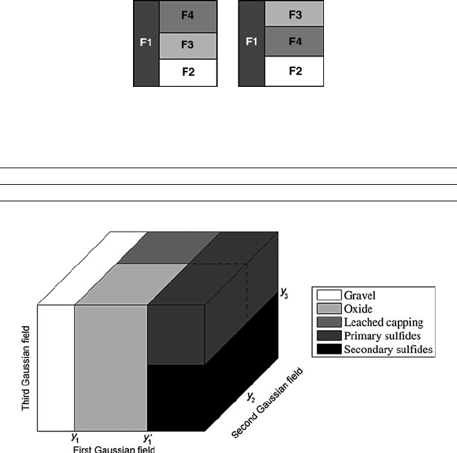
Fig. 5.7 Rectangle rocktype rules for four facies

80 5 Truncation and Thresholds

partitions. We have to make a choice, and then ﬁnd a criterion to help us do this.

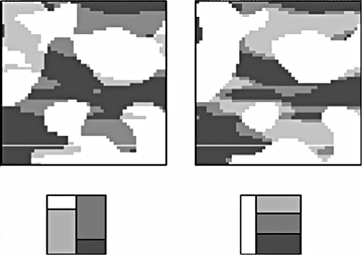
Figure5.8showsexamplesofsimulationscorrespondingtotwocasesfromFigure5.7.

We can see that the facies that touch each other in the rocktype rule are also in

contact in the simulation. This is a general rule when the proportions are constant,

and when the simulated ﬁeld is large enough to be statistically representative.

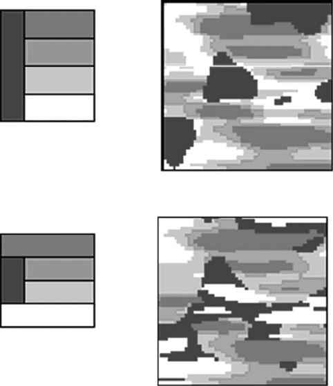
Thisruleis usuallysufﬁcient to choose thepartition if thereare only afewfacies,

but whe n the number increases we can ﬁnd several partitions which give the same

contact possibilities (Fig. 5.9). In that case, the shape of these contacts can also help

us.Wehavetodecidewhichgaussianfunctionwillguidetheshapeofwhichcontact.

When the proportions vary, some facies can disappear in some parts of the

simulated ﬁeld. In that case, the rocktype rule also varies, and the forbidden contact

will locally disappear.

Choice of the Correlation Matrix

With two gaussian functions, the correlation matrix which can be written as

S ¼

1 r

r 1



is consistent provided that 1 < r < 1. The values r ¼1 are also authorised,

but in that case it is better to work with only one gaussian function. The covariance

matrix must always be positive deﬁnite. With more than two gaussians, it would be

Fig. 5.8 Examples of simulation for two of the rocktype rules shown in Fig. 5.7

Idea Behind the Plurigaussian Method 81

virtually impossible to get a positive deﬁnite matrix just by picking values for the

terms. It is better to give a consistent model of relationships b etween the gaussians,

and then deduce a suitable covariance matrix from this. We will not go into more

detail here.

With two gaussian functions, once the rocktype rule is chosen, we still need to

know the M1 thresholds and the correlation, r, which gives M unknowns. So we

need M equations linking the unknowns to the proportion values. We have M

equations but they are not inde pendent because the partition automatically ensures

that the proportions sum to 1. As a consequence, we have more variables than

independent equations. The number of solutions is inﬁnite. Worse, these solutions

are not equivalent: they give rise to simulations that are quite different.

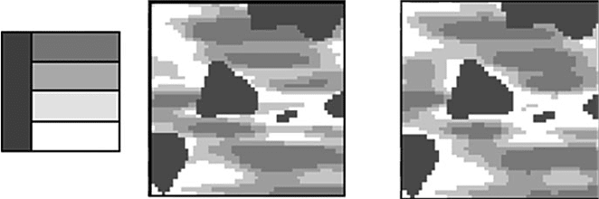
For example Fig. 5.10 shows two simulations obtained with the same partition

but different correlations, 0 and 0.6. The shape of the black facies is exactly the

same in both cases because the ﬁrst gaussian function is the same, but those of the

three other facies change. This is easiest to see on the white facies. In the right hand

simulation where the correlation is 0.6, the white tends to wrap around the black,

especially in the bottom left corner. In Chap. 8, we present a case study where

correlation will be used to drape one facies over algal bioherms.

Fig. 5.9 Examples of simulations with the same contacts, but with different rocktype rules

82 5 Truncation and Thresholds

The example given above shows that increasing the correlation coefﬁcient

introduces a border effect, which looks like the ordering effect we have with only

one gaussian function. This is the reason why we suggest choosing the value of the

correlation coefﬁcient arbitrarily, depending on whether we want to have a strong

border effect or not. Note that the correlation coefﬁcient is a property of the

gaussian functions: it will remain constant over the whole domain.

Calculating the Thresholds

When we have chosen the correlation coefﬁcient, we have M1 independent

equations of the form:

ðxÞ¼

gðz

;...;z

Þdz

...dz

;

where the D

are rectangles [t

i1

]  [s

i1

We have already seen that there are M1 independent thr esholds. This equation

system cannot be solved analytically, but iterative methods can give us the solution.

The trial and error method, testing successively all the thresholds, would be too

slow, because it does not automatically ensure the consistency of the partition in

rectangles.

Ingeneral,itisbettertoperformaglobal optimisation, mini mising for example

the global square error on the proportions. But in many cases, it is possible to

group the facies and work successively on one gaussian function, then the other

one(wemayhavetoiteratethis procedure). Figure 5.11 shows an example of

this. Here the trial and error method is very quick, because the partition is

automatically c onsistent. The partition we want to obtain is shown on the top

line. The sec o nd line s ho w s the ord er in which the thresholds are evaluated,

starting w ith the top block.

Fig. 5.10 Simulations with the same lithotype rule and different correlation coefﬁcients, r ¼ 0

and r ¼ 0.6

Idea Behind the Plurigaussian Method 83

Generalisation to Non-stationary Case

As for the truncated gaussian, non-stationarity is obtained via varying proportions.

This results in varying thresholds for both gaussian functions. The rocktype rule

must be given including all the facies, even if some of them can disappear locally.

When Simulations Show “Prohibited” Contacts

Sometimes simulations show contacts which do not exist in the rock type rule

diagram. In the stationary case, there are two possible reasons for this: one

(or more) of the gaussian functions is discontinuous, or the discretisation is too

coarse to show the continuity. This problem occurs much more often in the non-

stationary case. We will demonstrate this in the most common case of vertical non

stationarity for the truncated gaussian, but the same applies for horizontal

non stationarity and in the plurigaussian case.

When one facies disappears,the twofacies which shouldbe separated by it come

into direct contact. This is obvious when the local rock type rule is shown, but can

be forgotten when only the globa l rocktype rule is given. One consequence is that

the relative position of two facies which never appear at the same level is of no

importance (see Fig. 5.12). What must be taken into account is their relationship

with the other facies.

Two facies which are not in contact in the rock type rule can sometimes touch if

the proportions (and hence thethresholds) vary sharply between consecutive levels.

This is easy to see on the example below, where there are three facies : shale (F1),

shaly sandstone (F2) and sandstone (F3). On level 1, the proportions are respec-

tively 60%, 20% and 20%, which gives the thresholds t

¼ 0.25 and t

¼ 0.84.

On level 2, they are 20%, 20% and 60%, and so the thresholds are t

¼0.84,

¼0.25. The gaussian values between 0.25 and þ0.25 represent 20% of the

histogram. When the value simulated on level 1 is between 0.25 and 0.25 (which

corresponds to the facies shale), there is a high probability that on level 2 the

Fig. 5.11 Successive groupings to obtain the thresholds

84 5 Truncation and Thresholds

simulated gaussian value is located within the same interval. (This of course

depends on the variogram model). If that happens, the sandstone will be directly

in contact with the shale vertically below it (Table 5.3).

Higher Dimensional Rock-Type Rules

The rock-type rules pres ented up to this point have all been two dimensional, even

though higher dimensional rules are possible as Xu et al. (2006) showed. The

reasons for presenting only 2D rules are that they are easier to interpret and to

present in papers and reports and because we have not needed higher dimensional

Table 5.3 Schematic representation of the rocktype rules on two consecutive levels, respecting

the ordering in the threshold values

Level 2 Shale Shaly sandstones Sandstones

Level 1 Shale Shaly sandstones Sandstones

Fig. 5.12 Equivalent rocktype rules if F3 and F4 do not appear on the same level

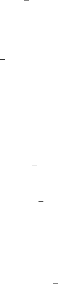
Fig. 5.13 3D rock-type rule used by Emery (2007a, b) for modelling ﬁve mineralogical domains

in a Chilean porphyry copper deposit: alluvial gravel, oxides, leached capping material, primary

and secondary sulphides. Reproduced with permission

Idea Behind the Plurigaussian Method 85

rules in any of our case-studies. Having said that, in a study of a Radomiro Tomic

porphyrycopper depositnorth of Calama City in Chile, Emery (2007b)encountered

a case where a 3D rule was required to represent the connections between the ﬁve

mineralogical domains of interest: alluvial gravels, leached capping, oxides, pri-

mary and secondary sulphides. The gravel are located near the surface and in

contact with the oxides and the leached capping but never the sulphides, but the

otherfour domains are in contact witheach other. A convenientway of representing

this situation is by using a 3D rule as shown in Fig. 5.13. Introducing a third

gaussian allows more ﬂexibility but complicates the variogram analysis.

86 5 Truncation and Thresholds

Chapter 6

Variograms and Structural Analysis

This chapter describes how to calculate experimental variograms for the facies

indicators and how to ﬁt models to them. The relationship between the facies

indicators and the underlying gaussian values has been given in Chap. 2.

In this chapter we will give the variogram equations in the case when we only

have constraints on facies but no other categorical variable or continuous function

in the data set.

The theoretical relation linking the variograms of the underlying gaussians and

those of the indicators is described. From this link we use a speciﬁc ﬁtting method:

rather than invert it, we use an indirect iterative procedure to ﬁt a variogram model.

But ﬁrst, we show how to calculate the experimental variograms for the facies

indicators.

Experimental Variograms and Cross-Variograms for Facies

In Chap. 2, the deﬁnition of the centred covariance of the indicators and its

relationship with the gaussian has been given. Here we consider the centred

variogram of the indicator of the facies F which is the tool used in most geostatis-

tical studies:

ðx;x þ h Þ¼

Var 1

ðxÞ1

ðx þ hÞ½

ðxÞ1

ðx þ hÞ½



 E1

ðxÞ1

ðx þ hÞ½ðÞ

When the facies indicators are second order stationary or intrinsic with constant

mean, the second term is zero and the formula simpliﬁes to:

(x, x þ h) ¼ g

(h) ¼

(x)  1

(x þ h)½



M. Armstrong et al., Plurigaussian Simulations in Geosciences,

DOI 10.1007/978-3-642-19607-2_6,

Springer-Verlag Berlin Heidelberg 2011

If the mean is not constant, it is still possible to deﬁne the non-centred variogram

ðx; x þ hÞ¼

ðxÞ1

ðx þ hÞ½



Centredvariogramandnon-centeredvariograms are equalwhenthe faciesindicators

aresecondorderstationaryorintrinsicwithconstantmean.Inthenon-stationarycase,

themeanE[1

(x)]cannotbe computedexperimentally.Inthisnon-stationary casewe

havenoalternativeto theexperimentalevaluation ofthenon-centredvariogram.Asa

consequence, we will compute the experimental non centred variogram in all cases.

Hence the formula for computing the experimental variogram for facies F is:



ðx, x þ hÞ¼

x

¼h

ðx

Þ1

ðx



where the data points x

and x

are separated by the vector h (possibly with a

tolerance). The summation is carried out over all the data pairs separated by this

distance, and N is the number of pairs. More information will be given later on how

to compute the experimental variogram in the non-stationary case.

In exactly the same way, the cross variogram for facies F

and F

is deﬁned as:

FiFj

ðx, x þ hÞ¼

(x)  1

(x þ h)½1

(x)  1

(x þ h)



Again, this corresponds to the centred (usual) cross-variogram in the second order

stationary case, and to a non-centred cross-variogram in the non stationary case.

Consequently the formula for the corresponding experimental cross-variogram is:



FiFj

ðx, x þ hÞ¼

x

¼h

ðx

Þ1

ðx



ðx

Þ1

ðx



Linking the Indicator Variograms to the Underlying Variograms

Wehave seen in Chap. 2 that the non centred covariance can be interpreted in terms

of probability: Covð1

xðÞ;1

x þ hðÞÞ¼Pðx 2 F

; x þ hðÞ2F

Variograms

From this equation, we can deduce that in the stationary case the variogram of the

indicator of facies F

can also be interpreted in terms of probability:

ðx,x þ hÞ¼

Px2 F

½+Pxþ h 2 F

½

 Px2 F

,xþ h 2 F

½

88 6 Variograms and Structural Analysis

If we consider the set of underlying gaussian functions Z(x) and the constraint C

(xÞ

which describes the link between Z(x) and the indicator 1

ðxÞ, this equation gives:

ðx,x þ hÞ¼

P Z(x) 2C

(x)½þP Z(x þ h) 2C

(x þ h)½fg

 P Z(x) 2C

ðxÞ;Z(x þ h) 2C

ðx þ hÞ½

Then

ðx,x þ hÞ¼

ðxÞþP

ðx þ hÞ



ðxþhÞ

ðxÞ

zðxÞ;zðxþhÞ

ðu, vÞdudv

Cross-Variograms

In the sameway as in Chap. 2, we showedthatthe cross-variogramcan be written as

ðx,x þ hÞ¼

E[1

(x)1

(x þ h)] þ E[1

(x)1

(x þ h)]



Hence

Fi Fj

ðx,x þ hÞ¼

PZxðÞ2C

xðÞ; Zxþ hðÞ2C

x þ hðÞ



þ PZxðÞ2C

xðÞ; Zxþ hðÞ2C

x þ hðÞ



and

Fi Fj

ðx,x þ hÞ¼

ðxþhÞ

ðxÞ

zðxÞ;zðxþhÞ

ðu,vÞdudv

ðxþhÞ

ðxÞ

zðxÞ;zðxþhÞ

ðu,vÞdu dv

;

In the next paragraphs, we will explain how to use these general equations in the

case of the truncated gaussian method (the vector Z(x) contains only a single

gaussian function) and of the classical plurigaussian method (the vector Z(x)

contains two or more gaussian functions).

Truncated Gaussian Method

In the truncated gaussian method, Z(x) 2C

ðxÞ can also be written t

i1

 ZðxÞ

ðxÞ where t

i1

and t

are the thresholds for facies F

Truncated Gaussian Method 89