Alligood K., Sauer T., Yorke J.A. Chaos: An Introduction to Dynamical Systems

Подождите немного. Документ загружается.

C ASCADES

Window size Period

ⴚ

| (

)

0.04506988 7 1.226617 1.635 0.27

0.00956120 7 1.299116 2.032 0.097

0.00197090 8 1.121835 2.229 0.0093

0.00084633 9 1.172384 2.245 0.0022

0.00049277 8 1.323307 2.248 0.00097

0.00033056 10 1.176765 2.244 0.0027

0.00032251 15 1.421811 1.637 0.27

0.00030118 9 1.402762 2.249 0.00036

0.00024599 13 1.353915 2.211 0.017

0.00022962 10 1.142882 2.246 0.0018

0.00022952 9 1.293955 2.246 0.0019

Table 12.3 Values of the ratio

for the H

enon map f(

) ⴝ (1 ⴚ

ⴙ

)

Data is drawn from windows in the range 1.12 ⬍ a ⬍ 1.43 with window widths

greater than 2 ⫻ 10

⫺4

for (a, x) near (a

), where p ⫽ p

⫹ p

. To be precise, q ⫽

⳵

f

⳵

)

and p ⫽ S

⫺1

⳵



⳵

a(a

The rescaling is given by the linear change of coordinates

y ⫽ qS(x ⫺ x

),u⫽⫺pqS

(a ⫺ a

In the terminology of the discussion above, the conjugacy H is deﬁned as

H(a, x) ⫽ (u, y) ⫽ (⫺pqS

(a ⫺ a

),qS(x ⫺ x

)).

Step 6 Let g(u, y) be the family of maps conjugate to f

(a, x)underthis

change of coordinates. From the expansion for f

in Step 5, show that

g(u, y) ⫽ y

⫺ u ⫹ O(S

⫺1

(|y|

⫹ |y||u| ⫹ |u|

)).

Since all cascades of the canonical map take place in a bounded region of (u, y)-

space, say (u, y) 僆 [⫺2.5, 2.5] ⫻ [⫺2.5, 2.5], conclude that g converges to the

canonical map as n →

⬁

The universality of the ratio R

appears to apply through a wide class

of chaotic systems, including multidimensional systems that contain cascades.

Table 12.3 shows a numerical study of periodic windows for the H

enon map

f(x

) ⫽ (1 ⫺ ax

⫹ x

, 0.3x

). The relative error between the calculated R

and

is seen to be typically quite small.

530

E XERCISES

12.1. Show that there are parameters a

and a

such that the quadratic family f

(x) ⫽

a ⫺ x

satisﬁes Hypotheses 12.7, the hypotheses of the Cascade Theorem.

12.2. Show that neither the quadratic family f

(x) ⫽ a ⫺ x

nor the logistic family g

(x) ⫽

ax(1 ⫺ x) has a period-two saddle node. Show, on the other hand, that each must

have a period-four saddle node.

12.3. Let g

(x) ⫽ 4x(1 ⫺ x), and let k be an odd number. Show that half the periodic

orbits of period k are regular repellers and half are ﬂip repellers. Similarly, for a map

that forms a hyperbolic horseshoe, half the periodic orbits of period k are regular

saddles and half are ﬂip saddles. Do the same results hold for any even k?

12.4. Let g denote either the logistic map g

or the horseshoe map. Use the following step

to show that for n ⱖ 24, at least 49% of the period n orbits of g are regular unstable

orbits and at least 49% are ﬂip unstable.

(a) Let N be the number of ﬁxed points of g

that are not period-n points. Show

that the proportion of one type of orbits (ﬂip or regular) is at least

n⫺1

⫺N

⫽

⫺

. In the remaining two parts we show that

⬍ .01, for n ⱖ 24.

(b) Show that the number N of ﬁxed points of g

of period less than n is at most

n 2

⫹ 2

n 3

⫹ 2

n 4

⫹⭈⭈⭈⫹2 ⱕ n2

n 2

⫺x 2

is decreasing for x ⬎

ln 2

, and that it is less

than .01 for n ⱖ 24.

12.5. Assume that a family of maps f

satisﬁes Hypotheses 12.7 of the Cascade Theorem.

Let p be a periodic orbit of period k at a ⫽ a

. Show that each such orbit p is

contained in a connected set of orbits that contains a cascade from period k.

The result follows from the Cascade Theorem if p is a regular unstable orbit.

We assume, therefore, that p is a ﬂip-unstable orbit.

(a) Let G be the following set of orbits: U

⫺

orbits of period k, and U

⫹

and S

orbits of period j, for all j ⱖ 2k. Show that there is a path of orbits of G through

each saddle node of period 2k or higher and through each period-doubling

bifurcation of period k or higher.

(b) Orient the branches of orbits in G to form a new type of “snake”, as follows:

→, U

⫹

←,andU

⫺

←. Show that Lemmas 12.10, 12.11, 12.12, 12.13, and

12.14 hold for these snakes to obtain the result. (Don’t forget to show that

period-k stable orbits are contained in the connected set of orbits.)

531

C ASCADES

☞ L AB V ISIT 12

Experimental Cascades

HE PERIOD-DOUBLING cascade is perhaps the most easily identiﬁable route

to chaos for a dynamical system. For this reason, experimental researchers at-

tempting to identify and study chaos in real systems are often drawn to look for

cascades. Here we will survey the ﬁndings of laboratories in Lille, France and

Berkeley, California. On the surface, the experiments have little in common—

one involves nonlinear optics, and the other an electrical circuit, but the cascades

that signal a transition to chaos are seen in both.

Scientists at the Laboratoire de Spectroscopie Hertzienne in Lille found period-

doubling cascades in two different laser systems. The ﬁrst, reported in 1991, was a

laser with modulated losses. The laser contains an electro-optic modulator

in the laser cavity, that modulates the amplitude of the laser output intensity.

The alternating current C(t) ⫽ a ⫹ b sin

␻

t applied to the modulator can be

controlled by the experimenter, and various behaviors are found as a, the dc bias,

and b, the modulation amplitude, are varied. The modulation frequency

␻

is ﬁxed

at 640 kHz, the resonance frequency of the device.

Fixing b and using a as a bifurcation parameter yields Figure 12.16 (also

shown as Color Plate 23). The modulation amplitude was set at b ⫽ 3V, and

the dc bias was varied from 60V at the left side of the picture to 460V at the

right side. To make this picture on the oscilloscope, the output intensity of the

laser was sampled 640,000 times per second, the modulation frequency. The

intensity makes a periodic orbit during each sampling period. A single value

branch in Figure 12.16 corresponds to a periodic intensity oscillation in step with

the modulation. The double branch that emanates from the single branch means

that the oscillation takes two periods of the modulation to repeat, and so on.

The orbit with doubled period is often called a subharmonic of the original orbit.

Lepers, C., Legrand, J., and Glorieux, P. 1991. Experimental investigation of the colli-

sion of Feigenbaum cascades in lasers. Physical Review A 43:2573–5.

Bielawski, S., Bouazaoui, M., Derozier, D., and Glorieux, P. 1993. Stabilization and

characterization of unstable steady states in a laser. Physical Review A 47:3276–9.

Kocarev, L., Halle, K. S., Eckert, K., and Chua, L. O. 1993. Experimental observation

of antimonotonicity in Chua’s circuit. Int. J. of Bifurcations and Chaos 3:1051–5.

532

L AB V ISIT 12

Figure 12.16 Period-doubling cascade from a CO

laser.

The dc bias of the modulator in the laser cavity is used as a bifurcation parameter, and

is increased from the left side of the diagram to the right. The resulting bifurcation

diagram of laser intensity shows a period-doubling cascade followed by a period-

halving cascade.

Cascades originate from both the right and the left, colliding in the chaotic region

in the middle. The orbits that are created in the initial cascade are systematically

destroyed as the dc bias is further increased, resulting in a reverse cascade.

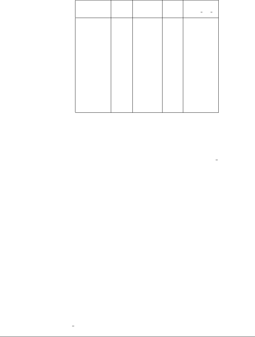
The same laboratory also produced Figure 12.17, which is a bifurcation

diagram of the power output of an optical-ﬁber laser. The active medium is a 5-

meter long silica ﬁber doped with 300 parts per million of trivalent neodymium,

a rare-earth metallic element. The medium is pumped by a laser diode. The input

power provided by the laser diode is the bifurcation parameter. Increasing the

power from 5.5 milliwatts (mW) to 7 mW results in the oscilloscope picture shown

here, which exhibits a period-doubling cascade ending in chaotic behavior for

large values of the power. By adjusting the tilting of the mirrors in this experiment,

various other nonlinear phenomena can be found, including Hopf bifurcations.

533

C ASCADES

Figure 12.17 Period-doubling cascade from an optical-ﬁber laser.

The pump power is increased from the left of the diagram to the right, resulting in

a bifurcation diagram showing a period-doubling cascade.

L. Chua’s laboratory in Berkeley was the setting for studies of bifurcation

phenomena in Chua’s circuit, which we introduced in Chapter 9. The bifurcation

parameter in this circuit was taken to be the capacitance C

across one of the

capacitors. (This parameter is proportional to 1 c

in the notation used for the

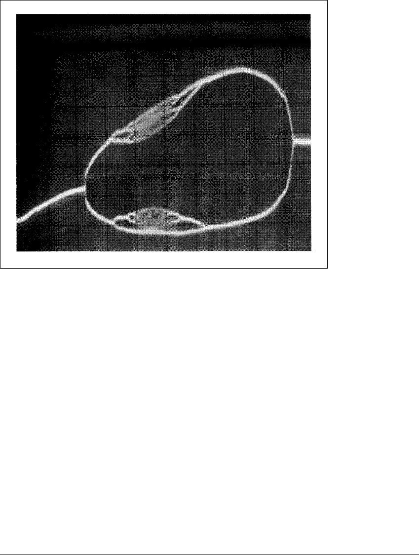
differential equations (9.6).) Figure 12.18(a) shows the readout of an oscilloscope

screen, exhibiting an experimental cascade as the parameter C

ranges from 3.92

nanoFarads (nF) to 4.72 nF. Each vertical division on the screen represents 200

millivolts.

Several different types of periodic and chaotic behavior can be seen in

this picture, including cascades, periodic windows (parameter ranges with only

periodic behavior), bubbles (collisions of cascades from the left and right) and

reverse bubbles (periodic windows with cascades emanating to both left and

right). A magniﬁcation of a part of the bifurcation diagram is shown in Figure

12.18(b). At least three odd-period windows are visible in this picture.

534

L AB V ISIT 12

Figure 12.18 Bifurcation diagrams for Chua’s circuit.

Voltage is graphed vertically as a function of the capacitance parameter C

.(a)

Period-doubling cascade followed by windows of period 5, 4, 3 and 2. (b) Magniﬁ-

cation of part of (a).

535

C ASCADES

Experimental bifurcation diagrams from both laboratories show antimono-

tonicity, the destruction of periodic orbits created in a cascade by a reverse

cascade. Although this does not occur for the one-dimensional logistic map, an-

timonotonicity is typical of higher-dimensional systems which contain cascades.

There are many other contributions to the scientiﬁc literature demonstrat-

ing period-doubling bifurcations and cascades in laboratory experiments. Many

occurred shortly after Feigenbaum’s published work in 1978.

In 1981, P. Linsay of MIT produced a cascade up to period 16 by varying the

driving voltage in a periodically-driven RLC circuit (Linsay, 1981). His estimate

of the Feigenbaum constant was 4.5 ⫾ 0.6. At about the same time, a group

of Italian researchers (Giglio, Musazzi, and Perini 1981), found a cascade up to

period 16 from a Rayleigh-B

enard experiment in a heated chamber ﬁlled with

water. Using the temperature gradient as a bifurcation parameter, they estimated

the Feigenbaum constant at approximately 4.3. Cascades were ﬁrst found in laser

experiments by (Arecchi et al., 1982). Another source with many interesting

examples of cascades and snakes in electronics is (Van Buskirk and Jeffries, 1985),

who studied networks of p-n junctions.

536

C HAPTER T HIRTEEN

State Reconstruction

fro m Da ta

HE STATE of a system is a primitive concept that uniﬁes the approach to many

sciences. In this chapter we will describe the way states can be inferred from

experimental measurements. In so doing we will revisit the Belousov-Zhabotinskii

chemistry experiment from Lab Visit 3, the Couette-Taylor physics experiment

from Lab Visit 4, and an example from insect physiology.

13.1 DELAY PLOTS FROM TIME SERIES

Our deﬁnition in Chapter 2 was that the state is all information necessary to

tell what the system will do next. For example, the state of a falling projectile

537

S TAT E R ECONSTRUCTION FROM DATA

consists of two numbers. Knowledge of its vertical height and velocity are enough

to predict where the projectile will be one second later.

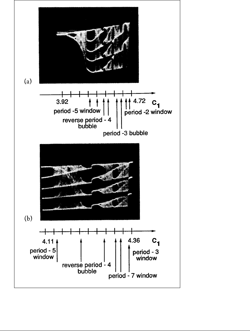
The states of a periodic motion form a simple closed curve. Figure 13.1(a)

shows a series of velocity measurements at a single point in the Couette-Taylor

experiment, as described in Lab Visit 4. A plot of a system measurement versus

time, as shown in Figure 13.1(a), is called a time series. For these experimental

settings, the system settles into a periodic motion, so the time series of velocity

measurements is periodic.

A useful graphical device in a situation like this is to plot the time series

using delay coordinates. In Figure 13.1(b) we plot each value of the time series

of velocities 兵S

其 versus a time-delayed version, by plotting (S

t⫺T

) for the ﬁxed

delay T ⫽ 0.03. This is called a delay-coordinate reconstruction, or delay plot.

In Figure 13.1, part (b) is made from part (a) as follows. At each time

t, a point is plotted in part (b) using the two velocities S(t)andS(t ⫺ 0.03).

At time t ⫽ 2, for example, the velocity is decreasing with S(2) ⫽ 800 and

S(1.97) ⫽ 1290. The point (800, 1290) is added to the delay plot. This is repeated

for all t for which recordings of the velocity were made, in this case, every 0.01

time unit. As these delay-coordinate points are plotted, they ﬁt together in a loop

that makes one revolution for each oscillation in the time series.

The interesting feature of a delay plot of periodic dynamics is that it can

reproduce the periodic orbit of the true system state space. If we imagine our

experiment to be ruled by k coupled autonomous differential equations, then the

state space is ⺢

. Each vector v represents a possible state of the experiment, and

800

1600

2400

0 2 4 6 8

Velocity

time

800

1600

2400

0 800 1600 2400

S(t-T)

S(t)

(a) (b)

Figure 13.1 Periodic Couette-Taylor experimental data.

(a) Time series of velocities from the experiment. (b) Delay plot of data from (a),

with time delay T ⫽ 0.03.

538

13.1 DELAY P LOTS FROM T IME S ERIES

by solving the differential equations, the state v(t) moves continuously through

the state space as time progresses.

We can imagine a set of coupled differential equations that governs the

behavior of the Couette-Taylor experiment, but it is not easy to write them

down. The state space dimension k would be very large; perhaps thousands of

differential equations modeling the movement of ﬂuid in small regions might

need to be tracked. This is called “modeling from ﬁrst principles”. In contrast to

the complicated differential equations of motion, the behavior we see in Figure

13.1 is fairly simple. Periodic motion means that trajectories trace out a one-

dimensional curve of states through ⺢

Of course, the idea of a real experiment being “governed” by a set of

equations is a ﬁction. The Couette-Taylor experiment is composed of metal, glass,

ﬂuid, an electric motor, and many other things, but not equations. Yet science has

been built largely on the success of mathematical models for real-world processes.

A set of differential equations, or a map, may model the process closely enough

to achieve useful goals.

Fundamental understanding of a scientiﬁc process can be achieved by build-

ing a dynamical model from ﬁrst principles. In the case of Couette-Taylor, the basic

principles include the equations of ﬂuid ﬂow between concentric cylinders, which

are far from completely understood on a fundamental level. The best differential

equation approximation for a general ﬂuid ﬂow is afforded by the Navier-Stokes

equations, whose solutions are known only approximately. In fact, at present it

has not been proved that solutions exist for all time for Navier-Stokes.

Can we answer questions about the dynamics of the system without un-

derstanding all details of the ﬁrst principles equations? Suppose we would like

to do time series prediction, for example. The problem is the following: Given

information about the time series of velocity at the present time t ⫽ 2, predict the

velocity at some time in the future, say 0.5 time units ahead. What information

about the present system conﬁguration do we need? Formally speaking, we need

to know the state—by deﬁnition, that is the information needed to tell the system

what to do next. But we don’t even know the dimension of the state space, let

alone what the differential equations are and how to solve them. To do time

series prediction, we will use the method of analogues. That means we will try

to identify what state the system is in, look to the past for similar states, and see

what ensued at those times.

How do we identify the present state at t ⫽ 2? Knowing that S(2) ⫽ 800

is not quite enough information. According to the time series Figure 13.1(a),

the velocity is 800 at two separate times; once when the velocity is decreasing,

and once when it is increasing. If we look 0.5 time units into the future from

the times that S ⫽ 800, we will get two quite different answers. We need a way

539