Alligood K., Sauer T., Yorke J.A. Chaos: An Introduction to Dynamical Systems
Подождите немного. Документ загружается.


M ATRIX A LGEBRA
There are three parts to the above classification. Let A bea2⫻ 2 real
matrix.
Fact 1. If A has real distinct eigenvalues a and b,orifA ⫽ aI,thenA ⬃
a 0
0 b
.
Proof: If A ⫽ aI we are done and a ⫽ b. If the eigenvalues are distinct,
then A is diagonalizable. To see this, choose eigenvectors v and x satisfying
Av ⫽ av and Ax ⫽ bx.Notethatv and x are not multiples of one another since
a ⫽ b, so that the matrix whose columns are v and x is invertible. Then
A
vx
⫽
av bx
⫽
vx
a 0
0 b
.
Now A is of form SDS
⫺1
,whereD ⫽ diag兵 a, b其.
Fact 2. If A has a repeated eigenvalue
⫽ a and A ⫽ aI,thenA ⬃
a 1
0 a
.
Proof: (A ⫺ aI)
2
⫽ 0. Since A ⫽ aI, there exists a vector x such that
v ⫽ (A ⫺ aI)x ⫽ 0. Then (A ⫺ aI)v ⫽ (A ⫺ aI)
2
x ⫽ 0, so v is an eigenvector
of A.Notethatv and x are not linearly dependent, since v is an eigenvector of A
and x is not. The facts Ax ⫽ ax ⫹ v and Av ⫽ av can be written
A
vx
⫽
vx
a 1
0 a
.
Fact 3. If A has eigenvalues a ⫾ bi,withb ⫽ 0, then A ⬃
a ⫺b
ba
.
Proof: (A ⫺ (a ⫹ bi)I)(A ⫺ (a ⫺ bi)I) ⫽ 0 can be rewritten as (A ⫺ aI)
2
⫽
⫺b
2
I.Letx be a (real) nonzero vector and define v ⫽
1
b
(A ⫺ aI)x,sothat(A ⫺
aI)v ⫽⫺bx.Sinceb ⫽ 0, v and x are not linearly dependent because x is not
an eigenvector of A. The equations Ax ⫽ bv ⫹ ax and Av ⫽ av ⫺ bx can be
rewritten
A
xv
⫽
xv
a ⫺b
ba
.
The similarity equivalence classes for m ⬎ 2 become a little more com-
plicated. Look up Jordan canonical form in a linear algebra book to investigate
further.
560

A.2 COORDINATE C HANGES
A.2 COORDINATE CHANGES
We work in two dimensions, although almost everything we say extends to higher
dimensions with minor changes. A vector in ⺢
2
can be represented in many dif-
ferent ways, depending on the coordinate system chosen. Choosing a coordinate
system is equivalent to choosing a basis of ⺢
2
; then the coordinates of a vector
are simply the coefficients that express the vector in that basis.
Consider the standard basis
B
1
⫽
1
0
,
0
1
and another basis
B
2
⫽
1
0
,
1
1
.
The coefficients of a general vector
x
1
x
2
are x
1
and x
2
in the basis B
1
, and are
x
1
⫺ x
2
and x
2
in the basis B
2
. This is because
x
1
1
0
⫹ x
2
0
1
⫽
x
1
x
2
⫽ (x
1
⫺ x
2
)
1
0
⫹ x
2
1
1
, (A.6)
or in matrix terms,
x
1
x
2
⫽
11
01
x
1
⫺ x
2
x
2
⫽ S
x
1
⫺ x
2
x
2
. (A.7)
This gives us a convenient rule of thumb. To get coordinates of a vector
in the second coordinate system, multiply the original coordinates by the matrix
S
⫺1
,whereS is a matrix whose columns are the coordinates of the second basis
vectors written in terms of the first basis. Therefore in retrospect, we could have
computed
x
1
⫺ x
2
x
2
⫽ S
⫺1
x
1
x
2
⫽
1 ⫺1
01
x
1
x
2
(A.8)
as the coordinates, in the second coordinate system B
2
, of the vector
x
1
x
2
in
the original coordinate system B
1
. For example, the new coordinates of
1
1
are
561

M ATRIX A LGEBRA
S
⫺1
1
1
⫽
0
1
, which is equivalent to the statement that
1
1
0
⫹ 1
0
1
⫽ 0
1
0
⫹ 1
1
1
. (A.9)
Now let F be a linear map on ⺢
2
. For a fixed basis (coordinate system), we
find a matrix representation for F by building a matrix whose columns are the
images of the basis vectors under F, expressed in that coordinate system.
For example, let F be the linear map that reflects vectors through the
diagonal line y ⫽ x. In the coordinate system B
1
the map F is represented by
A
1
⫽
01
10
(A.10)
since F
1
0
⫽
0
1
and F
0
1
⫽
1
0
. In the second coordinate system B
2
,
the vector F
1
0
⫽
0
1
has coordinates
S
⫺1
0
1
⫽
1 ⫺1
01
0
1
⫽
⫺1
1
,
and F fixes the other basis vector
1
1
,sothemapF is represented by
A
2
⫽
⫺10
11
. (A.11)
The matrix representation of the linear map F depends on the coordinate
system being used. What is the relation between the two representations? If x
is a vector in the first coordinate system, then S
⫺1
x gives the coordinates in
the second system. Then A
2
S
⫺1
x applies the map F,andSA
2
S
⫺1
x returns to
the original coordinate system. Since we could more directly accomplish this by
multiplying x by A
1
, we have discovered that
A
1
⫽ SA
2
S
⫺1
, (A.12)
or in other words, that A
1
and A
2
are similar matrices. Thus similar matrices are
those that represent the same map in different coordinate systems.
562

A.3 MATRIX T IMES C IRCLE E QUALS E LLIPSE
A.3 MATRIX TIMES CIRCLE EQUALS ELLIPSE
In this section we show that the image of the unit sphere in ⺢
m
under a linear
map is an ellipse, and we show how to find that ellipse.
Definition A.5 Let A be an m ⫻ n matrix. The transpose of A, denoted
A
T
,isthen ⫻ m matrix formed by changing the rows of A into columns. A square
matrix is symmetric if A
T
⫽ A.
In terms of matrix entries, A
T
ij
⫽ A
ji
. In particular, if the matrices are column
vectors x and y,thenx
T
y, using standard matrix multiplication, is the dot product,
or scalar product, of x and y. It can be checked that (AB)
T
⫽ B
T
A
T
.
It is a standard fact found in elementary matrix algebra books that for any
symmetric m ⫻ m matrix A with real entries, there is an orthonormal eigenbasis,
meaning that there exist m real-valued eigenvectors w
1
,...,w
m
of A satisfying
w
T
i
w
j
⫽ 0ifi ⫽ j,andw
T
i
w
i
⫽ 1, for 1 ⱕ i, j ⱕ m.
Now assume that A is an m ⫻ m matrix that is not necessarily symmetric.
The product A
T
A is symmetric (since (A
T
A)
T
⫽ A
T
(A
T
)
T
⫽ A
T
A), so it has an
orthogonal basis of eigenvectors. It turns out that the corresponding eigenvalues
must be nonnegative.
Lemma A.6 Let A be an m ⫻ m matrix. The eigenvalues of A
T
A are
nonnegative.
Proof: Let v be a unit eigenvector of A
T
A,andA
T
Av ⫽
v.Then
0 ⱕ |Av|
2
⫽ v
T
A
T
Av ⫽
v
T
v ⫽
.
These ideas lead to an interesting way to describe the result of multiplying
a vector by the matrix A. This approach involves the eigenvectors of A
T
A.Let
v
1
,...,v
m
denote the m unit eigenvectors of A
T
A, and denote the (nonnegative)
eigenvalues by s
2
1
ⱖ⭈⭈⭈ⱖs
2
m
. For 1 ⱕ i ⱕ m,defineu
i
by the equation s
i
u
i
⫽ Av
i
if s
i
⫽ 0; if s
i
⫽ 0, choose u
i
as an arbitrary unit vector subject to being orthogonal
to u
1
,...,u
i⫺1
. The reader should check that this choice implies that u
1
,...,u
n
are pairwise orthogonal unit vectors, and therefore another orthonormal basis of
⺢
m
. In fact, u
1
,...,u
n
forms an orthonormal eigenbasis of AA
T
.
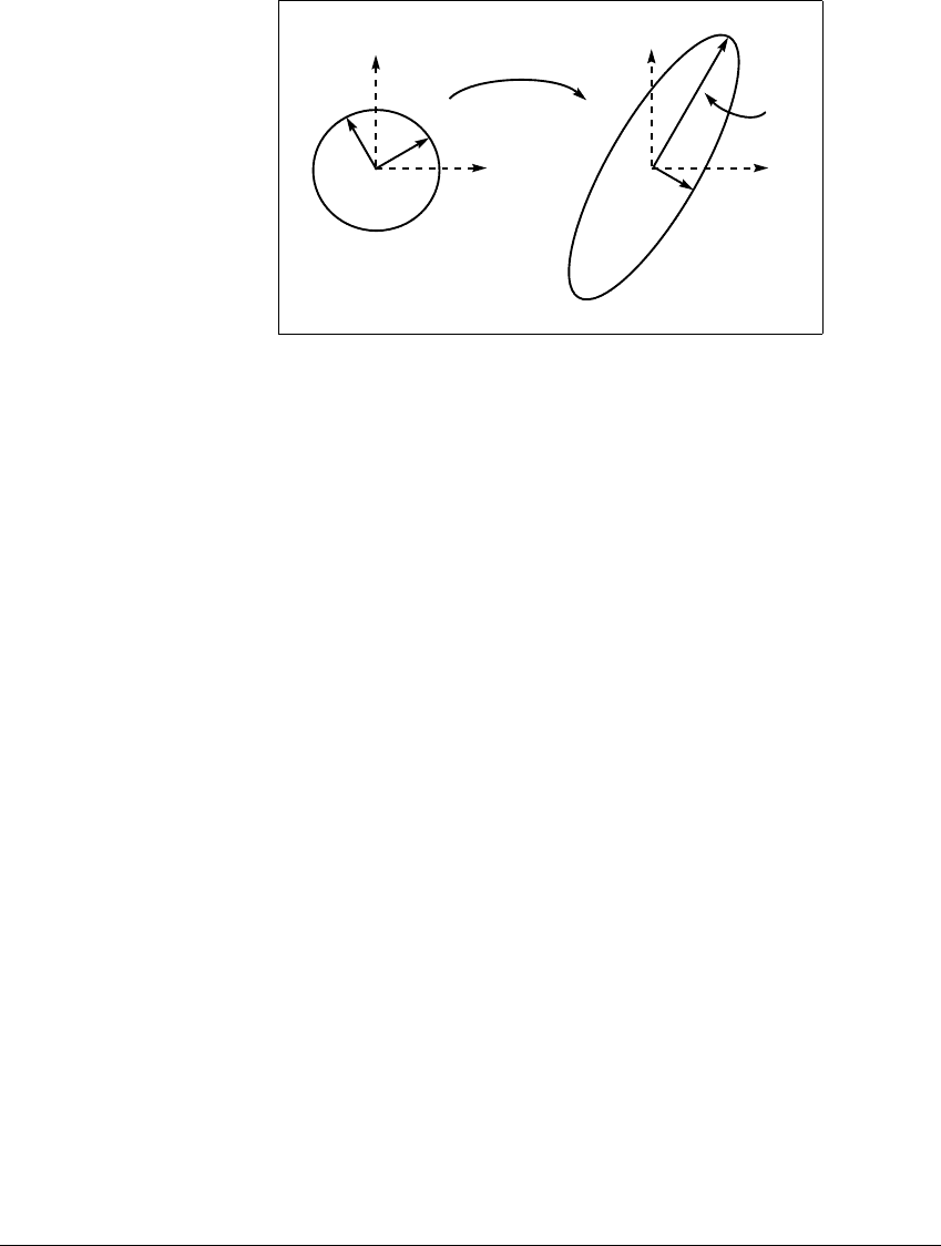
Figure A.1 shows a succinct view of the action of a matrix on the unit
circle in the m ⫽ 2 case. There is a pair of orthonormal coordinate systems, with
bases 兵v
1
, v
2
其 and 兵 u
1
, u
2
其, so that the matrix acts very simply: v
1
→ s
1
u
1
and
563
M ATRIX A LGEBRA
v
2
v
1
x
1
x
2
0
s
1
u
1
s
2
u
2
x
2
x
1
A
Figure A.1 The ellipse associated to a matrix.
Every 2 ⫻ 2 matrix A can be viewed in the following simple way. There is a coor-
dinate system 兵v
1
, v
2
其 for which A sends v
1
→ s
1
u
1
and v
2
→ s
2
u
2
,where兵u
1
, u
2
其
is another coordinate system and s
1
,s
2
are nonnegative numbers. Geometrically
speaking, a matrix A can be broken down into a dilation (stretching or shrinking
in orthogonal directions) followed by a rotation. This picture extends to
⺢
m
for an
m ⫻ m matrix.
v
2
→ s
2
u
2
. This means that the unit circle of vectors is mapped into an ellipse
with axes 兵s
1
u
1
,s
2
u
2
其. In order to find where Ax goes for a vector x, we can write
x ⫽ a
1
v
1
⫹ a
2
v
2
(where a
1
v
1
(resp. a
2
v
2
) is the projection of x onto the direction
v
1
(resp. v
2
)), and then Ax ⫽ a
1
s
1
u
1
⫹ a
2
s
2
u
2
. Summarizing, we have proved
Theorem A.7.
Theorem A.7 Let A be an m ⫻ m matrix. Then there exist two orthonormal
bases of ⺢
m
, 兵 v
1
,...,v
m
其 and 兵u
1
,...,u
m
其, and real numbers s
1
ⱖ ⭈⭈⭈ ⱖ s
m
ⱖ 0
such that Av
i
⫽ s
i
u
i
for 1 ⱕ i ⱕ m.
We conclude from this theorem that the image of the unit sphere of vectors
is an ellipsoid of vectors, centered at the origin, with semi-major axes s
i
u
i
.
The foregoing discussion is sometimes summarized in a single matrix equa-
tion. Define S to be a diagonal matrix whose entries are s
1
ⱖ⭈⭈⭈ⱖs
m
ⱖ 0. Define
U to be the matrix whose columns are u
1
,...,u
m
,andV to be the matrix whose
columns are v
1
,...,v
m
. Notice that USV
T
v
i
⫽ s
i
u
i
for i ⫽ 1,...,m. Since the
matrices A and USV
T
agree on the basis v
1
,...,v
m
, they are identical m ⫻ m
matrices. The equation
A ⫽ USV
T
(A.13)
564

A.3 MATRIX T IMES C IRCLE E QUALS E LLIPSE
is called the singular value decomposition of A,andthes
i
are called the singular
values. The matrices U and V are called orthogonal matrices because they satisfy
U
T
U ⫽ I and V
T
V ⫽ I. Orthogonal matrices correspond geometrically to rigid
body transformations like rotations and reflections.
565

A PPENDIX B
Computer Solution
of ODEs
S
OME ORDINARY DIFFERENTIAL EQUATIONS can be solved explicitly. The initial
value problem
˙
x ⫽ ax
x(0) ⫽ x
0
(B.1)
has solution
x(t) ⫽ x
0
e
at
. (B.2)
The solution can be found using the separation of variables technique introduced
in Chapter 7. The fact that the problem yields an explicit solution makes it
atypical among differential equations. In the large majority of cases, there does
567

C OMPUTER S OLUTION OF ODES
not exist an expression for the solution of the initial value problem in terms of
elementary functions. In these cases, we have no choice but to use the computer
to approximate a solution.
B.1 ODE SOLVERS
A computational method for producing an approximate solution to an initial
value problem (IVP) is called an ODE solver. Figure B.1(a) shows how a typical
ODE solver works. Starting with the initial value x
0
, the method calculates
approximate values of the solution x(t)onagrid兵t
0
,t
1
,...,t
n
其.
The simplest ODE solver is the Euler method. For the initial value problem
˙
x ⫽ f(t, x)
x(t
0
) ⫽ x
0
, (B.3)
the Euler method produces approximations by an iterative formula. Choosing
a step size h ⬎ 0 determines a grid 兵t
0
,t
0
⫹ h, t
0
⫹ 2h,...其. Denote the correct
values of the solution x(t)byx
n
⫽ x(t
n
). The Euler method approximations at
the grid points t
n
⫽ t
0
⫹ nh are given by
w
0
⫽ x
0
w
n⫹1
⫽ w
n
⫹ hf(t
n
,w
n
) for n ⱖ 1. (B.4)
Each w
n
is the Euler method approximation for the value x
n
⫽ x(t
n
)ofthe
solution.
It is easy to write a simple program implementing the Euler method. The
code fragment
w[0] = w0;
t[0] = t0;
for(n=0;n<=N;n++){
t[n+1] = t[n]+h;
w[n+1] = w[n]+h*f(t[n],w[n]);
}
together with a defined function f from the differential equation will generate
the grid of points 兵t
n
其 along with the approximate solutions 兵w
n
其 at those points.
Remember to set the step size h. The smaller the value for h, the smaller the error,
which is the subject of the next section.
A far more powerful method that requires just a few more lines is the
Runge-Kutta method of order 4. A code fragment implementing this method is
568

B.1 ODE SOLVERS
w[0] = x0;
t[0] = t0;
for(n=0;n<=N;n++){
t[n+1] = t[n]+h;
k1 = h*f(t[n],w[n]);
k2 = h*f(t[n]+h/2,w[n]+k1/2);
k3 = h*f(t[n]+h/2,w[n]+k2/2);
k4 = h*f(t[n+1],w[n]+k3);
w[n+1] = w[n]+(k1 + 2*k2 + 2*k3 + k4)/6;
}
To run a simulation of a three-dimensional system such as the Lorenz at-
tractor, it is necessary to implement Runge-Kutta for a system of three differential
equations. This involves using the above formulas for each of the three variables
in parallel. A possible implementation:
wx[0] = x0;
wy[0] = y0;
wz[0] = z0;
t[0] = t0;
for(n=0;n<=N;n++){
t[n+1] = t[n]+h;
kx1 = h*fx(t[n],wx[n],wy[n],wz[n]);
ky1 = h*fy(t[n],wx[n],wy[n],wz[n]);
kz1 = h*fz(t[n],wx[n],wy[n],wz[n]);
kx2 = h*fx(t[n]+h/2,wx[n]+kx1/2,wy[n]+ky1/2,wz[n]+kz1/2);
ky2 = h*fy(t[n]+h/2,wx[n]+kx1/2,wy[n]+ky1/2,wz[n]+kz1/2);
kz2 = h*fz(t[n]+h/2,wx[n]+kx1/2,wy[n]+ky1/2,wz[n]+kz1/2);
kx3 = h*fx(t[n]+h/2,wx[n]+kx2/2,wy[n]+ky2/2,wz[n]+kz2/2);
ky3 = h*fy(t[n]+h/2,wx[n]+kx2/2,wy[n]+ky2/2,wz[n]+kz2/2);
kz3 = h*fz(t[n]+h/2,wx[n]+kx2/2,wy[n]+ky2/2,wz[n]+kz2/2);
kx4 = h*fx(t[n+1],wx[n]+kx3,wy[n]+ky3,wz[n]+kz3);
ky4 = h*fy(t[n+1],wx[n]+kx3,wy[n]+ky3,wz[n]+kz3);
kz4 = h*fz(t[n+1],wx[n]+kx3,wy[n]+ky3,wz[n]+kz3);
wx[n+1] = wx[n]+(kx1 + 2*kx2 + 2*kx3 + kx4)/6;
wy[n+1] = wy[n]+(ky1 + 2*ky2 + 2*ky3 + ky4)/6;
wz[n+1] = wz[n]+(kz1 + 2*kz2 + 2*kz3 + kz4)/6;
}
Here it is necessary to define one function for each of the differential equations:
fx(t,x,y,z) = 10.0*(y-x);
fy(t,x,y,z) = -x*z + 28*x - y;
fz(t,x,y,z) = x*y - (8/3)*z;
569

C OMPUTER S OLUTION OF ODES
This code can be economized significantly using object-oriented programming
ideas, which we will not pursue here. Any other three-dimensional system can
be approximated using this code, by changing the function calls fx,fy and fz.
Higher-dimensional systems require only a simple extension to more variables.
So far we have given no advice on the choice of step size h. The smaller h
is, the better the computer approximation will be. For the Lorenz equations, the
choice h ⬇ 10
⫺2
is small enough to produce representative trajectories.
Coding time can be reduced to a minimum by using a software package
with ODE solvers available. Matlab is a general-purpose mathematics software
package whose program ode45is an implementation of the Runge-Kutta method,
in which step size h is set automatically and monitored to keep error within
reasonable bounds. To use this method one needs only to create a file named f.m
containing the differential equations; ode45does the rest. Type help ode45in
Matlab for full details. Other generally available mathematical software routines
such as Maple and Mathematica have similar capabilities.
Finally, the software package Dynamics has a built-in graphical user interface
that runs Runge-Kutta simulations of the Lorenz equations and several other
systems with no programming required. See (Nusse and Yorke, 1995).
B.2 ERROR IN NUMERICAL INTEGRATION
As suggested in Figure B.1(a), there is usually a difference between the true
solution x(t) to the IVP and the approximation. Denote the total error at t
n
by
E
n
⫽ x
n
⫺ w
n
. Error results from the fact that an approximation is being made by
discretizing the differential equation. For Euler’s method, this occurs by replacing
˙
x by (x
n⫹1
⫺ x
n
) h in moving from (B.3) to (B.4).
The initial value problem (B.1) has an explicit solution, so we can work
out the exact error to illustrate what is going on. Set t
0
⫽ 0, so that t
n
⫽ nh.The
Euler method formula from (B.4) is
w
0
⫽ x
0
w
n⫹1
⫽ w
n
⫹ ahw
n
for n ⱖ 0. (B.5)
For example, assume a ⫽ 1, x
0
⫽ 1, and the stepsize is set at h ⫽ 0.1. Then w
1
⫽
1 ⫹ 0.1 ⫽ 1.1, which is not too far from the correct answer x
1
⫽ e
0.1
⬇ 1.105.
The error made in one step of the Euler method is ⬇ 0.005. A formula for the
one-step error is e
1
⫽ w
0
(e
ah
⫺ (1 ⫹ ah)).
570