Alligood K., Sauer T., Yorke J.A. Chaos: An Introduction to Dynamical Systems
Подождите немного. Документ загружается.


C HALLENGE 4
Step 7 The previous step says that L(
⑀
) is roughtly proportional to
⑀
p
for
small
⑀
. This quantifies the fact that the larger the fractal dimension of J, the
greater the uncertainty in prediction. For example, suppose boxdim (J) ⫽ 0.9, so
that p ⫽ 0.1. How much of a reduction in measurement accuracy
⑀
is necessary
to reduce the total length of
⑀
-uncertain points by a factor of two?
Step 8 Prove a two-dimensional version. Assume that J is a fractal basin
boundary in ⺢
2
, and that each point in J is in the boundary of at least two basins.
Show that the total area A(
⑀
)of
⑀
-uncertain points satisfies the formula
lim
⑀
→0
(ln A(
⑀
)) (ln
⑀
) ⫽ p,
where p ⫽ 2⫺ boxdim(J), and C is a constant.
Postscript. The subject of this Challenge is the damaging effect on final state
prediction due to fractal basin boundaries in one-dimensional maps. The characterization
of J in Step 4 means that each point in J is in the boundary of each of the two basins. Basin
boundaries of two-dimensional maps are even more intricate and interesting—they form
the subject of Challenge 10. There we investigate points that are simultaneously in the
boundary of three basins.
185

F RACTALS
E XERCISES
4.1. (a) Establish a one-to-one correspondence between the portion of the middle-
third Cantor set in [0, 1 3] and the entire Cantor set.
(b) Repeat part (a), replacing [0, 1 3] by [19 27, 20 27].
4.2. Consider the middle-half Cantor set K(4) formed by deleting the middle half of
each subinterval instead of the middle third.
(a) What is the total length of the subintervals removed from [0,1]?
(b) What numbers in [0, 1] belong to K(4)?
(c) Show that 1 5isinK(4). What about 17 21?
(d) Find the length and box-counting dimension of the middle-half Cantor set.
(e) Let S be the set of initial conditions that never map outside of the unit
interval for the tent map T
a
, as in Exercise T4.6. For what value of the parameter
a is S ⫽ K(4)?
4.3. Let T be the tent map with a ⫽ 2.
(a) Prove that rational numbers map to rational numbers, and irrational num-
bers map to irrationals.
(b) Prove that all periodic points are rational.
(c) Prove that there are uncountably many nonperiodic points.
4.4. Show that the set of rational numbers has measure zero.
4.5. Let
ˆ
K be the subset of the Cantor set K whose ternary expansion does not end in a
repeating 2. Show that there is a one-to-one correspondence between
ˆ
K and [0, 1].
Thus K is uncountable because it contains the uncountable set
ˆ
K.
4.6. Let K be the middle-third Cantor set.
(a) A point x is a limit point of a set S if every neighborhood of x contains a
point of S aside from x. A set is closed if it contains all of its limit points. Show
that K is a closed set.
(b) A set S is perfect if it is closed and if each point of S is a limit point of S.
Show that K is a perfect set. A perfect subset of
⺢ that contains no intervals of
positive length is called a Cantor set.
(c) Let S be an arbitrary Cantor set in
⺢. Show that there is a one-to-one
correspondence between S and K(3). In fact a correspondence can be chosen so
that if s, t 僆 S are associated with s
,t
僆 K(3), respectively, then s ⬍ t implies
s
⬍ t
; that is, the correspondence preserves order.
4.7. Find the box-counting dimension of:
(a) The middle 1 5 Cantor set.
186
E XERCISES
(b) The Sierpinski carpet.
4.8. Find the box-counting dimension of the set of endpoints of removed intervals for
the middle-third Cantor set K.
4.9. Another way to find the attracting set of the Sierpinski gasket of Computer Experi-
ment 4.1 is to iterate the following process. Remove the upper right one-quarter of
the unit square. For each of the remaining three quarters, remove the upper right
quarter; for each of the remaining 9 squares, remove the upper right quarter, and
so on. (a) Find the box-counting dimension of the resulting gasket. (b) Show that
the gasket consists of all pairs (x, y) such that for each n,thenth bit of the binary
representations of x and y are not both 1.
4.10. Let A and B be bounded subsets of
⺢.LetA ⫻ B be the set of points (x, y)inthe
plane such that x is in A and y is in B. Show that boxdim(A ⫻ B) ⫽ boxdim(A) ⫹
boxdim(B).
4.11. (a) True or false: The box-counting dimension of a finite union of sets is the
maximum of the box-counting dimensions of the sets. Justify your answer.
(b) Same question for countable unions, assuming that it is bounded.
4.12. This problem shows that countably infinite sets S can have either zero or nonzero
box-counting dimension.
(a) Let S ⫽ 兵0其 傼 兵1, 1 2, 1 3, 1 4,...其. Show that boxdim(S) ⫽ 0.5.
(b) Let S ⫽ 兵0其 傼 兵1, 1 2, 1 4, 1 8,...其. Show that boxdim(S) ⫽ 0.
4.13. Generalize the previous problem by finding a formula for boxdim(S):
(a) S ⫽ 兵0其 傼 兵n
⫺p
: n ⫽ 1, 2,...其,where0⬍ p.
(b) S ⫽ 兵0其 傼 兵p
⫺n
: n ⫽ 0, 1, 2,...其,where1⬍ p.
4.14. The time-2
map of the forced damped pendulum was introduced in Chapter 2.
The following table was made by counting boxes needed to cover the chaotic orbit
of the pendulum, using various box sizes. Two hundred million iterations of the
time-2
map were made. Find an estimate of the boxdim of this set. If you know
some statistics, say what you can about the accuracy of your estimate.
Box size Boxes hit
2
⫺2
111
2
⫺3
327
2
⫺4
939
2
⫺5
2702
2
⫺6
7839
2
⫺7
22229
2
⫺8
62566
2
⫺9
178040
187
F RACTALS
☞ L AB V ISIT 4
Fractal Dimension in Experiments
F
INDING THE fractal dimension of an attractor measured in the laboratory
requires careful experimental technique. Fractal structure by its nature covers
many length scales, so the construction of a “clean” experiment, where only
the phenomenon under investigation will be gathered as data, is important. This
ideal can never be achieved exactly in a laboratory. For this reason, computational
techniques which “filter” unwanted noise from the measured data can sometimes
help.
A consortium of experts in laboratory physics and data filtering, from Ger-
many and Switzerland, combined forces to produce careful estimates of fractal
dimension for two experimental chaotic attractors. The first experiment is the
hydrodynamic characteristics of a fluid caught between rotating cylinders, called
the Taylor-Couette flow. The second is an NMR laser which is being driven by a
sinusoidal input.
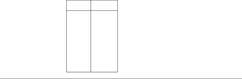
The Taylor-Couette apparatus is shown in Figure 4.19. The outside glass
cylinder, which has a diameter of about 2 inches, is fixed, and the inner steel
h
d
Figure 4.19 Setup of the Taylor-Couette flow experiment.
As the inner steel cylinder rotates, the viscous fluid between the cylinders undergoes
complicated but organized motion.
Kantz, H., Schreiber, T., Hoffman, I., Buzug, T., Pfister, G., Flepp, L. G., Simonet, J.,
Badii, R., Brun, E., 1993. Nonlinear noise reduction: A case study on experimental
data. Physical Review E 48:1529-1538.
188
L AB V ISIT 4
cylinder, which has a diameter of 1 inch, rotates at a constant rate. Silicon oil,
a viscous fluid, fills the region between cylinders. Care was taken to regulate the
temperature of the oil, so that it was constant to within 0.01
◦
C. The speed of
the rotating inner cylinder could be controlled to within one part in 10,000. As
shown in the figure, the top of the chamber is not flat, but set at a tiny angle,
to destroy unwanted effects due to symmetries of the boundary conditions. The
top surface is movable so that the “aspect ratio” h d can be varied between 0 and
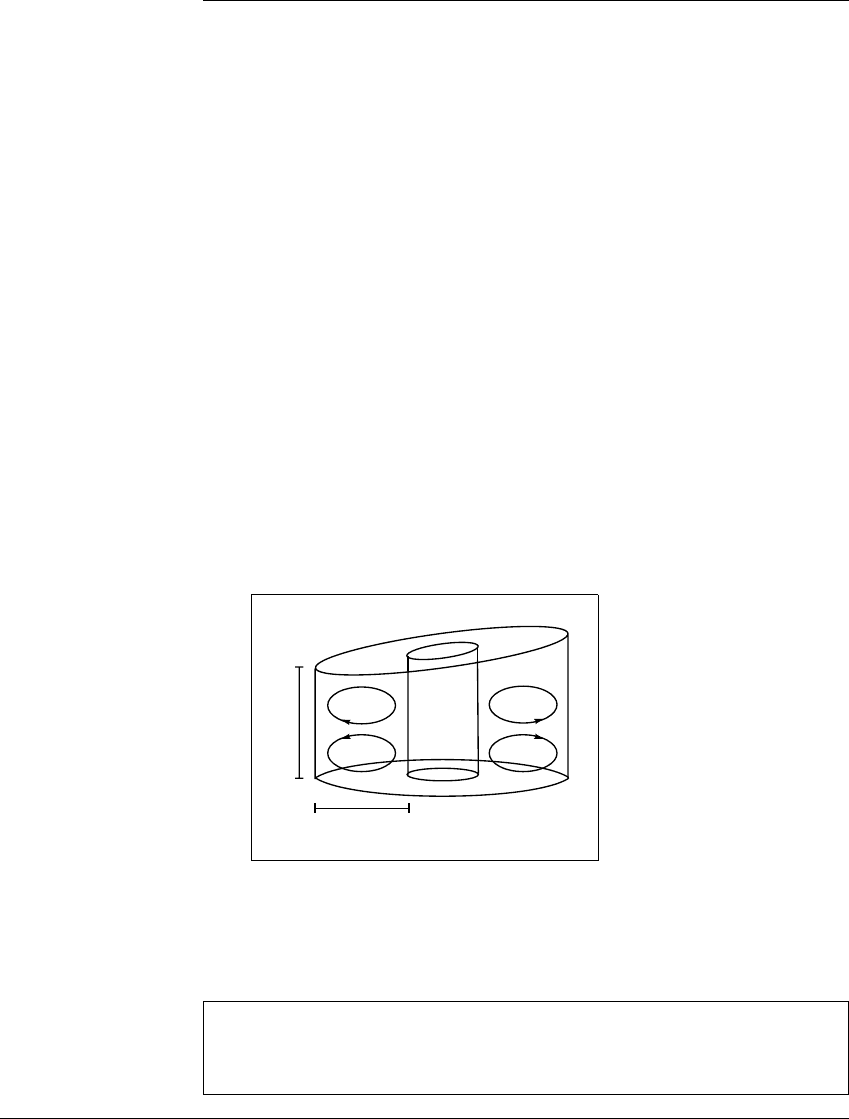
Figure 4.20 The Taylor-Couette data and its dimension.
(a) A two-dimensional projection of the reconstructed attractor obtained after
filtering the experimental data. The time delay is T ⫽ 5. (b) Slope estimates of the
correlation sum. There are 19 curves, each corresponding to correlation dimension
estimates for an embedding dimension between 2 and 20. The 32,000 points plotted
in Figure 4.20(a) were used in the left half, and only 2000 points in the right half, for
comparison. The conclusion is that the correlation dimension is approximately 3.
189
F RACTALS
more than 10, although an aspect ratio of 0.374 was used for the plots shown
here.
The measured quantity is the velocity of the fluid at a fixed location in the
chamber. Light-scattering particles were mixed into the silicon oil fluid, and their
velocities could be tracked with high precision using a laser Doppler anemometer.
The velocity was sampled every 0.02 seconds.
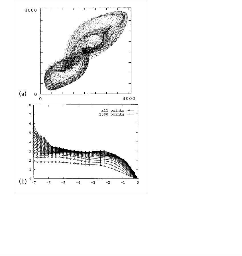
Figure 4.21 The NMR laser data and its estimated dimension.
(a) Time-delay plot of a Poincar
´
e section of the NMR laser data. About 39,000
returns to the Poincar
´
e surface were counted and plotted. (b) Estimated slopes
from the correlation sum from the data in (a). The researchers report a correlation
dimension estimate of 1.5.
190

L AB V ISIT 4
Figure 4.20(a) shows a time-delay plot of the velocity of the Taylor-Couette
flow experiment. We saw a first example of a time-delay plot in Figure 3.19; we
will give a more comprehensive treatment in Chapter 13. For now, we recall that
a time-delay reconstruction of a data series (Y
t
),whichinthiscaseconsistsof
the Taylor-Couette velocity readings, is constructed by plotting vectors of form
(y
t
,y
t⫹T
, ..., y
t⫹(m⫺1)T
)in⺢
m
. The delay used in Figure 4.20(a) is T ⫽ 0.1
seconds, or 5 sampling units. The dimensionality of the time-delay plot, m,is
called the embedding dimension. In Figure 4.20(a), m ⫽ 2.
Once the set of vectors is plotted in ⺢
m
, its properties can be analyzed as
if it were an orbit of a dynamical system. In fact, it turns out that many of the
dynamical properties of the orbit of the Taylor-Couette system that is producing
the measurements are passed along to the set of time-delay vectors, as explained in
Chapter 13. In particular, as first suggested in (Grassberger and Procaccia, 1983),
the correlation dimension can be found by computing the correlation function
of (4.9) using the time-delay vectors, and approximating the slope of a line as in
Figure 4.17.
The resulting slope approximations for the line log C(
⑀
) log
⑀
, which are
the correlation dimension estimates as
⑀
→ 0, are graphed in Figure 4.20(b)
as a function of log
⑀
. The several curves correspond to computations of the
correlation functions in embedding dimensions 2, 3, ..., 20. Here it is evident
how evaluation of a limit as
⑀
→ 0 can be a challenge when experimental data
is involved. We want to see the trend toward smaller
⑀
, the left end of Figure
4.20(b). However, the effects of experimental uncertainties such as measurement
noise are most strongly felt at very small scales. The range 2
⫺5
⬍
⑀
⬍ 2
⫺2
shows
agreement on a dimension of about 3.
The ingredients of a laser are the radiating particles (atoms, electrons,
nuclei, etc.) and the electromagnetic field which they create. An external energy
source causes a “population inversion” of the particles, meaning that the higher-
energy states of the particles are more heavily populated than the lower ones.
The laser cavity acts as a resonant chamber, which provides feedback for the laser
field, causing coherence in the excitation of the particles. For the ruby NMR laser
used in this experiment, the signal is a essentially a voltage measurement across
a capacitor in the laser cavity.
The laser output was sampled at a rate of 1365 Hz (1365 times per second).
A Poincar
´
e section was taken from this data, reducing the effective sampling
rate to 91 Hz. The time-delay plot of the resulting 39,000 intersections with
the Poincar
´
e surface is shown in Figure 4.21(a). The researchers estimate the
noise level to be about 1.1%. After filtering, the best estimate for the correlation
dimension is about 1.5, as shown in Figure 4.21(b).
191

C HAPTER F IVE
Chaos in
Two-Dimensional Maps
T
HE CONCEPTS of Lyapunov numbers and Lyapunov exponents can be extended
to maps on ⺢
m
for m ⱖ 1. In the one-dimensional case, the idea is to measure
separation rates of nearby points along the real line. In higher dimensions, the
local behavior of the dynamics may vary with the direction. Nearby points may
be moving apart along one direction, and moving together along another.
In this chapter we will explain the definition of Lyapunov numbers and
Lyapunov exponents in higher dimensions, in order to develop a definition of
chaos in terms of them. Following that, we will extend the Fixed-Point Theorems
of the one-dimensional case to higher dimensions, and investigate prototypical
examples of chaotic systems such as the baker map and the Smale horseshoe.
193
C HAOS IN T WO-DIMENSIONAL M APS
5.1 LYAPUNOV EXPONENTS
For a map on ⺢
m
, each orbit has m Lyapunov numbers, which measure the
rates of separation from the current orbit point along m orthogonal directions.
These directions are determined by the dynamics of the map. The first will be
the direction along which the separation between nearby points is the greatest
(or which is least contracting, if the map is contracting in all directions). The
second will be the direction of greatest separation, chosen from all directions
perpendicular to the first. The third will have the most stretching of all directions
perpendicular to the first two directions, and so on. The stretching factors in each
of these chosen directions are the Lyapunov numbers of the orbit.
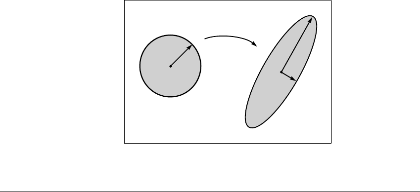
Figures 5.1 and 5.2 illustrate this concept pictorially. Consider a sphere of
small radius centered on the first point v
0
of the orbit. If we examine the image
f(S) of the small sphere under one iteration of the map, we see an approximately
ellipsoidal shape, with long axes along expanding directions for f and short axes
along contracting directions.
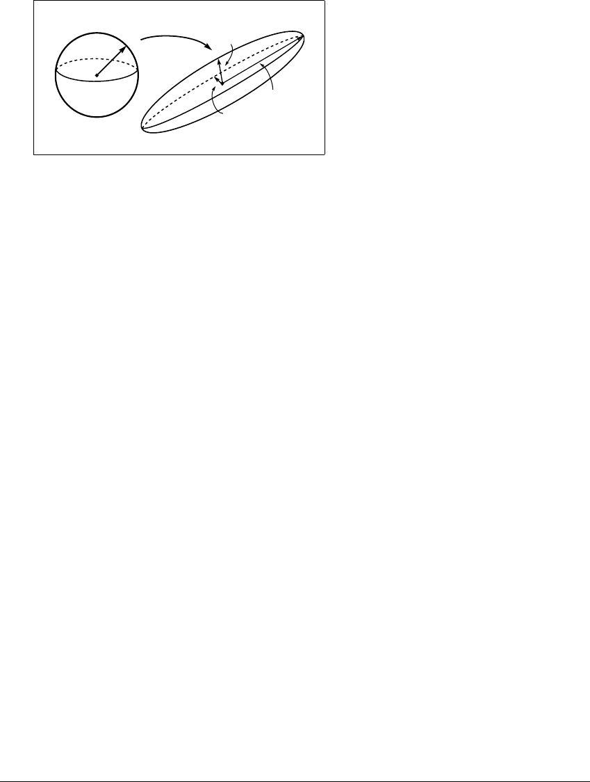
After n iterates of the map f, the small sphere will have evolved into a
longer and thinner ellipsoid-like object. The per-iterate changes of the axes of
this image “ellipsoid” are the Lyapunov numbers. They quantify the amount of
stretching and shrinking due to the dynamics near the orbit beginning at v
0
.The
natural logarithm of each Lyapunov number is a Lyapunov exponent.
For the formal definition, replace the small sphere about v
0
and the map f
by the unit sphere N and the first derivative matrix Df(v
0
), since we are interested
in the infinitesimal behavior near v
0
.LetJ
n
⫽ Df
n
(v
0
) denote the first derivative
1
f
n
(v
0
)
f
n
v
0
r
1
n
r
2
n
Figure 5.1 Evolution of an initial infinitesimal disk.
After n iterates of a two-dimensional map, the disk is mapped into an ellipse.
194
5.1 LYAP U NOV E XPONENTS
r
2
r
1
r
3
n
n
n
1
v
0
f
n
Figure 5.2 A three-dimensional version of Figure 5.1.
A small ball and its image after n iterates, for a three-dimensional map.
matrix of the nth iterate of f.ThenJ
n
N will be an ellipsoid with m orthogonal
axes. This is because for every matrix A, the image AN is necessarily an ellipsoid,
as we saw in Chapter 2. The axes will be longer than 1 in expanding directions
of f
n
(v
0
), and shorter than 1 in contracting directions, as shown in Figure 5.1.
The m average multiplicative expansion rates of the m orthogonal axes are the
Lyapunov numbers.
Definition 5.1 Let f be a smooth map on ⺢
m
,letJ
n
⫽ Df
n
(v
0
), and
for k ⫽ 1,...,m,letr
n
k
be the length of the kth longest orthogonal axis of the
ellipsoid J
n
N for an orbit with initial point v
0
.Thenr
n
k
measures the contraction
or expansion near the orbit of v
0
during the first n iterations. The kth Lyapunov
number of v
0
is defined by
L
k
⫽ lim
n→
⬁
(r
n
k
)
1 n
,
if this limit exists. The kth Lyapunov exponent of v
0
is h
k
⫽ ln L
k
. Notice that
we have built into the definition the property that L
1
ⱖ L
2
ⱖ ⭈⭈⭈ ⱖ L
m
and
h
1
ⱖ h
2
ⱖ ⭈⭈⭈ ⱖ h
m
.
If N is the unit sphere in ⺢
m
and A is an m ⫻ m matrix, then the orthogonal
axes of the ellipsoid AN can be computed in a straightforward way, as we showed
in Theorem 2.24 of Chapter 2. The lengths of the axes are the square roots of
the m eigenvalues of the matrix AA
T
, and the axis directions are given by the m
corresponding orthonormal eigenvectors.
Using the concept of Lyapunov exponent, we can extend the definition of
chaotic orbit to orbits of higher dimensional maps. For technical reasons which
we describe later (Example 5.5), we will require that no Lyapunov exponent is
exactly zero for a chaotic orbit.
195