Alfred DeMaris - Regression with Social Data, Modeling Continuous and Limited Response Variables
Подождите немного. Документ загружается.

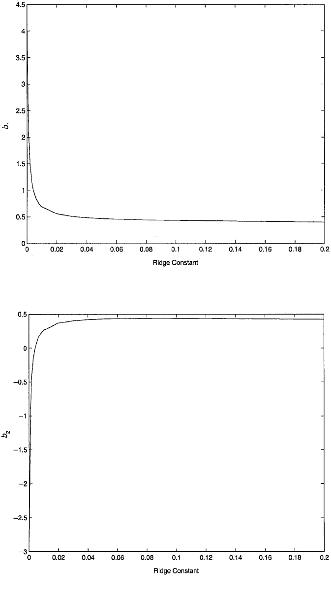
Figure 6.5 Ridge trace for the coefficient of triceps skinfold thickness (b
1
) in the regression model for
body fat.
Figure 6.6 Ridge trace for the coefficient of thigh circumference (b
2
) in the regression model for
body fat.
c06.qxd 8/27/2004 2:53 PM Page 235
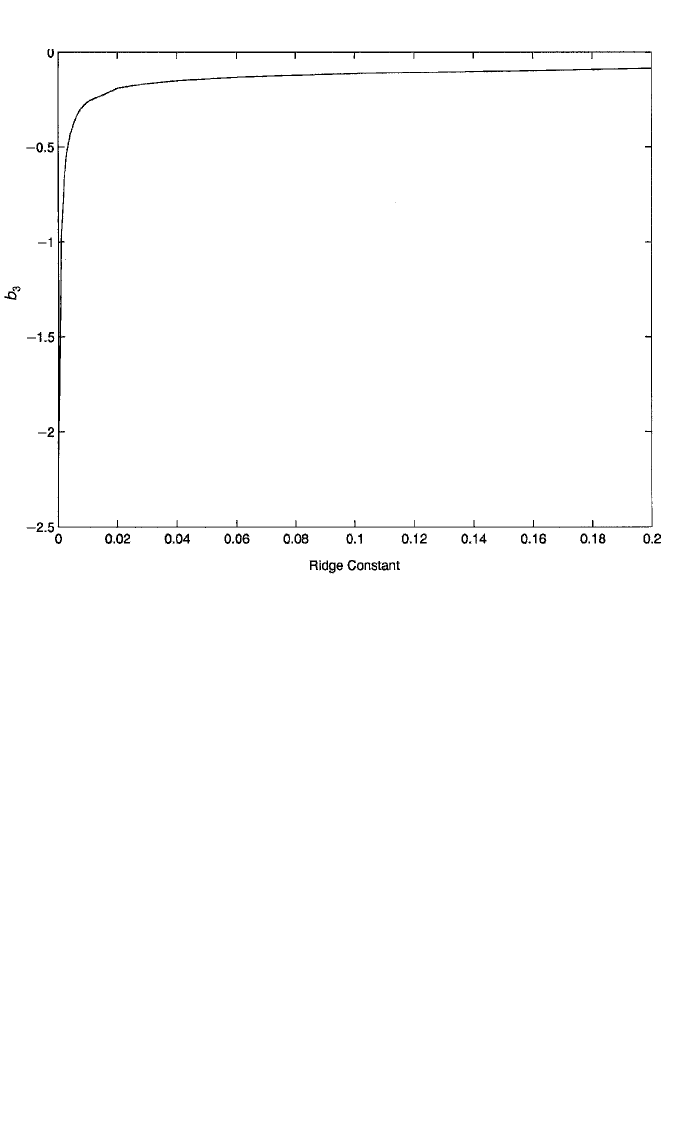
Each of the plots suggests that the coefficients stabilize right around δ .02, and
hence, this is the value chosen for the ridge constant. Notice in Figure 6.6, in partic-
ular, that the coefficient for thigh circumference changes sign from negative to pos-
itive very quickly as δ increases away from zero, and then remains positive. As
expected, this suggests that a greater thigh circumference is associated with more,
rather than less, body fat. The ridge regression estimates are shown in the “ridge
estimator” column of panel A of Table 6.7. These are the unstandardized estimates
and so can be compared to the OLS estimates in the first column. All have been
reduced markedly in magnitude, consistent with the expected reduction in the
coefficients once the multicollinearity problem has been addressed.
The ridge traces for male- and female age, male- and female age at the beginning
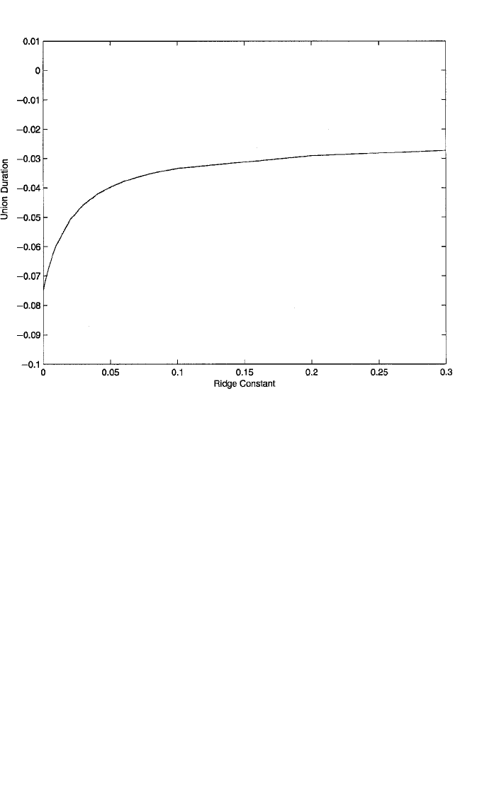
of the union, and union duration for the NSFH data are shown in Figures 6.8 to 6.12.
As these are the most problematic variables in the analysis, I choose a value of δ
based on an attempt to stabilize their effects. In this case, all of the graphs point
toward the value of .05 for δ, so this is the ridge constant that was chosen. Notice that
the coefficient for female age changes from positive to negative as δ moves away from
zero. Again, a negative effect was expected theoretically. Of the five plots, Figure
6.12, showing the trend in the coefficient for union duration, appears to evince the
most dramatic change. The ridge estimates are shown in the “ridge estimator” column
236 ADVANCED ISSUES IN MULTIPLE REGRESSION
Figure 6.7 Ridge trace for the coefficient of midarm circumference (b
3
) in the regression model for
body fat.
c06.qxd 8/27/2004 2:53 PM Page 236
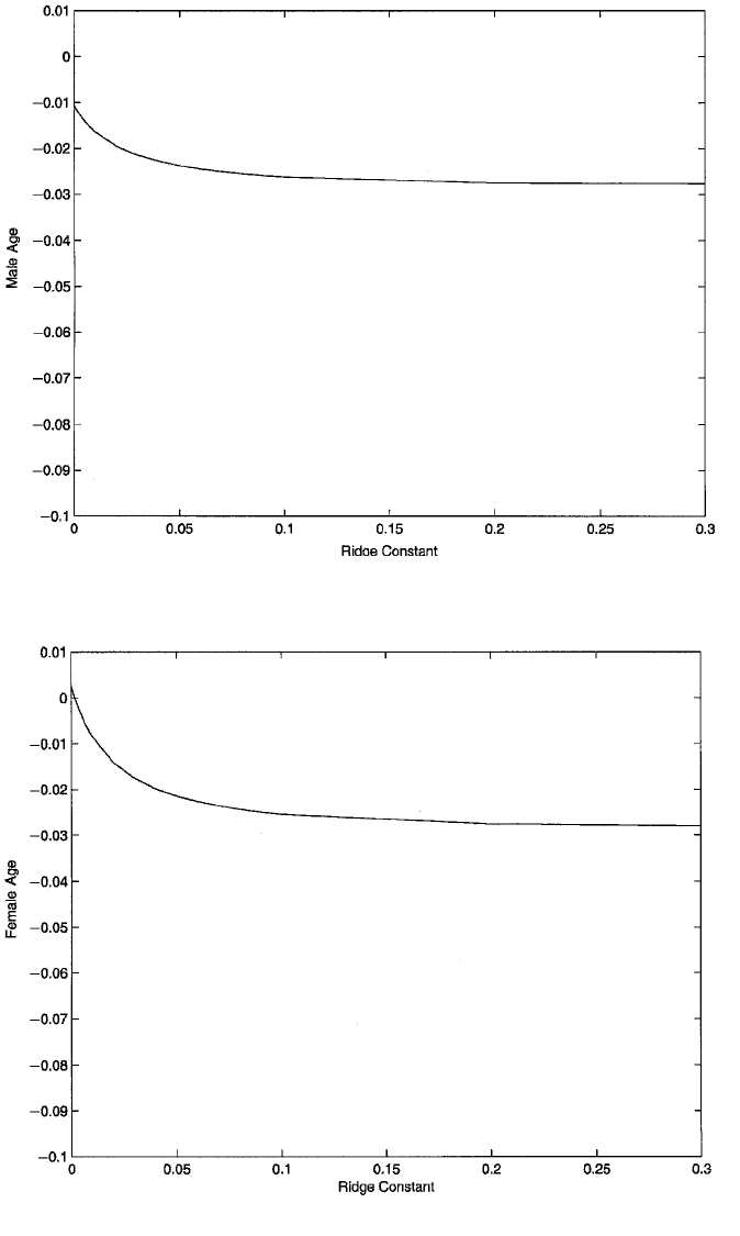
Figure 6.8 Ridge trace for the coefficient of male age in the regression model for couple disagreement.
Figure 6.9 Ridge trace for the coefficient of female age in the regression model for couple disagreement.
c06.qxd 8/27/2004 2:53 PM Page 237
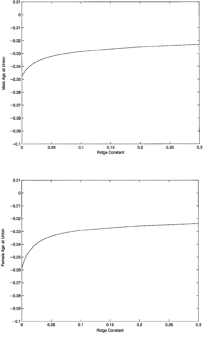
Figure 6.10 Ridge trace for the coefficient of male age at union in the regression model for couple dis-
agreement.
Figure 6.11 Ridge trace for the coefficient of female age at union in the regression model for couple
disagreement.
c06.qxd 8/27/2004 2:53 PM Page 238
of panel A of Table 6.8. Again, these are the unstandardized coefficients. In this case,
there is some shrinkage in all of the coefficients, compared to the OLS estimates, but
the changes are nowhere near as pronounced as in Table 6.7. The most notable change
is the aforesaid reversal of sign for the effect of female age.
Principal Components Regression. Principal components regression, also called
regression on principal components, gets its name from the fact that the n scores on
the K independent variables can be linearly transformed into a comparable set of
scores on K principal components. However, the principal components have the
property that they are orthogonal to each other. Each principal component is a
weighted sum of all K of the original variables. Moreover, the principal components
contain all of the variance of the original variables, but the first J K principal com-
ponents typically account for the bulk of that variance. The variance of the jth com-
ponent is equal to the jth eigenvalue of R
xx
. So components associated with small
eigenvalues contribute very little to the data and as a result, can be omitted from the
analysis. As the small eigenvalues are associated with linear dependencies, this
omission also greatly reduces the impact of those linear dependencies on the design
matrix. Standard treatments of principal components regression (e.g., Jolliffe, 1986;
Myers, 1986) usually develop the technique by writing the regression model in terms
of the principal components.
REGRESSION DIAGNOSTICS II: MULTICOLLINEARITY 239
Figure 6.12 Ridge trace for the coefficient of union duration in the regression model for couple dis-
agreement.
c06.qxd 8/27/2004 2:53 PM Page 239

Instead, I employ an alternative, but equivalent development that is more consistent
with the notion of altering the correlation matrix, as discussed above with respect to
ridge regression. Once again, we rely on the spectral decomposition of the design
matrix to understand the procedure. Recall that the design matrix can be decomposed
as R
xx
冱λ
j
u
j
u
j
, which is the sum of K rank 1 matrices, each of the form λ
j
u
j
u
j
(that
these matrices only have rank 1 is left as a proof for the reader). However, if λ
j
is small,
the contribution of λ
j
u
j
u
j
to R
xx
is relatively insignificant. But it is at the same time the
contribution that is associated with a linear dependency, so it is also troublesome to
include (as we see below). In principal components regression we simply leave this
contribution out of R
xx
(and its inverse, R
xx
1
) when calculating the regression estimates.
To see the benefits of this, let’s return to our simple two-regressor example used ear-
lier. For the design matrix in which X
1
and X
2
are correlated .995, the eigenvalues are
1.995 and .005, with corresponding eigenvectors u
1
[.7071 .7071] and u
2
[.7071
.7071]. The spectral decomposition of R
xx
shows that it is the sum of two parts:
λ
1
u
1
u
1
1.995
冤冥
[.7071 .7071]
冤冥
(6.17)
and
λ
2
u
2
u
2
.005
冤冥
[.7071 .7071]
冤冥
. (6.18)
The reader can easily verify that the sum of the rightmost matrices in (6.17) and
(6.18) is R
xx
. But notice that the matrix in (6.17), which I refer to as the reduced cor-
relation matrix and denote as R
red
, almost perfectly reproduces R
xx
, while the con-
tribution of the matrix in (6.18) is almost negligible. However, the decomposition of
R
xx
1
, following equation (6.13), shows that its two parts are
λ
1
1
u
1
u
1
′ .5013
冤冥
[.7071 .7071]
冤冥
(6.19)
and
λ
1
2
u
2
u
2
′ 200
冤冥
[.7071 .7071]
冤冥
. (6.20)
Adding the rightmost expressions in (6.19) and (6.20) gives us R
xx
1
, as shown above.
Here it is clear that the contribution of the second eigenvalue, in the form of its
inverse, and associated eigenvector are what “blow up” R
xx
1
. Therefore, in con-
structing “R
xx
1
,” we simply omit the matrix in (6.20). I’m using quotation marks here
since the reduced form of R
xx
1
, which I now denote R
red
, is not actually the inverse
of R
red
(which can easily be verified by noting that R
red
R
red
I). In fact, R
red
is not
invertible, since it is a 2 2 matrix with rank 1, as is immediately evident—there is
only one independent vector present. In general, R
red
is not invertible because it is
K K but is the sum of fewer than K rank 1 matrices. As the rank of a summed
matrix is no greater than the sum of the ranks of its component matrices (Searle,
1982), the rank of R
red
is always less than K, and therefore R
red
cannot have an
100 100
100 100
.7071
.7071
.2506 .2506
.2506 .2506
.7071
.7071
.0025 .0025
.0025 .0025
.7071
.7071
.9975 .9975
.9975 .9975
.7071
.7071
240 ADVANCED ISSUES IN MULTIPLE REGRESSION
c06.qxd 8/27/2004 2:53 PM Page 240

inverse. Consequently, I refer to R
red
in (6.19) as the pseudoinverse of R
red
. The stan-
dardized principal components coefficients are therefore
b
s
pc
R
red
r
xy
冤冥冤冥
冤冥
.
Although these are not quite as close to the true values of .25 and .15 as are the ridge
estimates, they represent a vast improvement over the OLS estimates.
In general, then, the principal components estimator of
ββ
s
is of the form b
s
pc
R
red
r
xy
, where
R
red
冱
J
i1
λ
1
i
u
i
u
i
and J K. Some authors recommend using the percentage of variance accounted for
by the J retained components as a guide to how many components to omit (e.g., Hadi
and Ling, 1998). However, typically, dropping the last component, which is associ-
ated with the smallest eigenvalue, will be sufficient. As with ridge regression, the
bias of the principal components estimator is easy to see, since
E(b
s
pc
) E(R
_
red
r
xy
) R
_
red
1
n
Z E(y
z
) R
_
red
1
n
ZZ
ββ
s
R
_
red
R
xx
ββ
s
ββ
s
.
Body Fat and NSFH Data, Revisited. The last column in panel A of Tables 6.7 and
6.8 presents the unstandardized principal components estimates for the body fat and
NSFH data, respectively. Notice that the principal components estimates are quite
close to the ridge regression estimates, and both are substantially different from the
OLS estimates for the body fat data. For the NSFH data, all of the estimates, whether
OLS, ridge, or principal components, are fairly similar. Perhaps the key substantive
difference between OLS and the other estimators are that the latter have more intu-
itive signs for the effect of thigh circumference in the body fat data and for the effect
of female age in the NSFH data. Again, the primary limitation with the latter esti-
mators is that inferences to the population parameters cannot be made. On the other
hand, the ridge and principal components estimators are probably closer than the
OLS coefficients to the true values of the parameters. It should be mentioned that not
all software makes these two techniques available to the analyst. SAS offers both
estimators as options to the OLS regression procedure, invoked using the keywords
RIDGE (for ridge regression) and PCOMIT (for principal components regression).
Concluding Comments. Although I confine my discussion of influential observa-
tions as well as collinearity problems and remedies to this chapter, these issues apply
to all generalized linear models. Influence diagnostics have been devised for tech-
niques such as logistic regression (Pregibon, 1981) and are included in such software
packages as SAS. Collinearity problems can plague any model that employs multiple
regressors; however, not all procedures offer collinearity diagnostics. On the other
hand, multicollinearity is strictly a problem in the design matrix and does not depend
on the nature of the link to the response. Therefore, it can always be diagnosed with
.2
.2
.40925
.38875
.2506 .2506
.2506 .2506
REGRESSION DIAGNOSTICS II: MULTICOLLINEARITY 241
c06.qxd 8/27/2004 2:53 PM Page 241

an OLS procedure that provides collinearity diagnostics, which most of them do. One
simply needs to code the dependent variable in some manner that is consistent with
the use of OLS. Versions of ridge and principal components regression have been
developed for logistic regression (see, e.g., Barker and Brown, 2001; Schaefer, 1986),
suggesting that such techniques should become more widely available for other gen-
eralized linear models in the future.
EXERCISES
6.1 Suppose that we have a population of N 4 cases. Let X be a matrix with
columns x
1
[1 2 4 8] and x
2
[2 1 3 4]. Suppose further that
σ
x
1
2.681 and σ
x
2
1.118. Also, let C be the centering matrix with dimen-
sions C
44
I
44
1
4
J
44
.
(a) Show that Z CXD
1/2
is the matrix of standardized variable scores for
these four cases, where D
1/2
is a diagonal matrix with elements 1/σ
x
i
.
(b) Calculate the correlation matrix using R
xx
(1/n)ZZ.
6.2 Prove that the inverse of D
c
i
is D
1/c
i
for i 1,2,...,n.
6.3 Show that A 冱λ
j
u
j
u
j
UD
λ
U.
6.4 Prove that if λ
j
are the eigenvalues of A, 1/λ
j
are the eigenvalues of A
1
.
(Hint: Start with the spectral decomposition of A and then take the inverse of
both sides of the equation.)
6.5 Let r
x
1
x
2
.675 and show that VIF
1
and VIF
2
are the diagonal elements of R
1
xx
.
6.6 Prove that MSQE(θ
ˆ
) V(θ
ˆ
) [B(θ
ˆ
)]
2
. (Hint: Start with the definition of MSQE;
let Eθ
ˆ
E(θ
ˆ
) for economy of notation, then subtract and add this term from
the expression inside parentheses and expand the expression.)
6.7 Prove that the matrix λuu has only rank 1, for any scalar λ and any vector u.
6.8 Verify that, in general, for any square matrix A, tr(cA) c tr(A), for any
scalar c.
6.9 For the following data:
Case XY Case XY
1 22 6 612
2 3 3 7 9 5.5
336 8 98
4 6 4.5 9 15 2
567
242 ADVANCED ISSUES IN MULTIPLE REGRESSION
c06.qxd 8/27/2004 2:53 PM Page 242

Do the following using a calculator:
(a) Calculate h
ii
for all nine cases.
(b) For case 9, calculate t
i
, dffits
i
, dfbetas
ji
for the slope of the SLR and
Cook’s D
i
. Note that another formula for Cook’s D is (Neter et al.,
1985)
D
i
pM
e
2
S
i
E
(1
h
i
h
i
ii
)
2
.
Also, for dfbetas
ji
, use σ
ˆ
b
1
from the regression that omits case 9.
6.10 Let Z
1
z
11
z
2
11
and let Z
2
[z
21
z
22
] represent matrices of standardized
variable scores (i.e., assume that Z
2
11
is standardized after being created from
the square of Z
11
) and suppose that the following model (in standardized
coefficients) characterizes the data:
Y
z
.25Z
11
.01Z
2
11
.3Z
21
.25Z
22
ε
y
,
Z
21
.2Z
2
11
ε
21
,
Z
22
.15Z
2
11
ε
22
,
Cov(Z
11
,Z
2
11
) .8,
Cov(Z
11
,ε
y
) Cov(Z
11
,ε
21
) Cov(Z
11
,ε
22
)
Cov(Z
2
11
,ε
y
) Cov(Z
2
11
,ε
21
) Cov(Z
2
11
,ε
22
) 0.
(a) If the analyst, instead, estimates y
z
Z
1
ββ
s
1
υ, where υ Z
2
ββ
s
2
εε
y
,give
the value of E(b
s
1
). [Hint: First, note that E(b
s
1
)
ββ
s
1
r
1
11
r
12
ββ
s
2
, where
r
1
11
r
12
β
s
2
is the bias in b
s
1
and
r
11
冤冥
and
r
12
冤冥
.
Then use covariance algebra to derive all unknown correlations (recall that the
covariance between standardized variables is their correlation), and do the
appropriate matrix operations.]
(b) Interpret the nature of the bias in the sample quadratic term.
6.11 Let Z
1
[z
11
z
12
cp], where CP Z
11
Z
12
, and let Z
2
[z
21
z
22
]. Suppose
further that all variables, including CP, are standardized. (Note: Normally, we
don’t standardize quadratic or cross-product terms; rather, they are formed as
products of standardized variables; see Aiken and West, 1991. However, we
Cov(Z
11
,Z
22
)
Cov(Z
2
11
,Z
22
)
Cov(Z
11
,Z
21
)
Cov(Z
2
11
,Z
21
)
Cov(Z
11
,Z
2
11
)
1
1
Cov(Z
11
,Z
2
11
)
EXERCISES 243
c06.qxd 8/27/2004 2:53 PM Page 243

do so here to simplify the covariance algebra.) Suppose that the following
model (in standardized coefficients) characterizes the data:
Y
z
.25Z
11
.15Z
12
.10CP .35Z
21
.3Z
22
ε
y
,
Z
21
.2CP ε
21
,
Z
22
.1CP ε
22,
Cov(Z
11
,Z
12
) .45,
Cov(Z
11
,CP) .85,
Cov(Z
12
,CP) .90,
and the covariances of Z
11
, Z
12
, and CP, with all equation errors equal zero.
(a) If the analyst, instead, estimates Y
z
Z
1
ββ
s
1
υυ
, where υ Z
2
ββ
s
2
εε
y
,give
the value of E(b
s
1
). (Hint: Follow the hint for Exercise 6.10.)
(b) Interpret the nature of the bias in the sample estimate of the coefficient of
the cross-product term (i.e., CP).
The following information is for Exercises 6.12 and 6.13: Suppose that the true
model for Y is β
1
Z
1
β
2
Z
2
ε, where all observed variables are standardized.
Suppose, further, that the sample correlation matrix is R
xx
冤冥
and
the sample vector of correlations of the regressors with Y is r
xy
冤冥
. Note also that the eigenvalues of R
xx
are λ
1
1.997 and λ
2
.003, while
the eigenvectors are u
1
冤冥
and u
2
冤冥
.
6.12 Estimate
ββ
s
冤冥
using OLS. Then perform a ridge regression using the
following values for the ridge constant: .05, .10, .15, .20, and .25. You will
have five different pairs of coefficient estimates. What appears to be the best
ridge constant based on the changes in the coefficients?
6.13 Conduct a principal components regression for the data in Exercise 6.12.
The following information is for Exercises 6.14 and 6.15: In the model
y* X*
ββ
s
εε
*
, the spectral decomposition of the 4 4 correlation matrix, R
xx
,
results in the following:
D
λ
冤冥
,
0
.
0
.00091806
.
.
.0689
0
0
.9996
2.9305
0
.
0
β
s
1
β
s
2
.7071
.7071
.7071
.7071
.7192
.6786
.997
1
1
.997
244 ADVANCED ISSUES IN MULTIPLE REGRESSION
c06.qxd 8/27/2004 2:53 PM Page 244
