Zdunkowski W., Trautmann T., Bott A. Radiation in the atmosphere: A course in Theoretical Meteorology
Подождите немного. Документ загружается.


6.2 The two-stream radiative transfer equation 165
yields
2π
1
0
b(−µ)I (τ, µ)dµ =
b
+
µ
+
E
+
,2π
1
0
b(−µ)I (τ, −µ)dµ =
b
−
µ
−
E
−
(6.34)
Equations (6.32) and (6.34) can now be employed to eliminate all expressions
in (6.29) and (6.30) which contain the radiance I (τ,µ). The resulting differential
equations for the up- and downward flux densities can be written as a 2 × 2 matrix
differential equation which reads
dE
dτ
= A · E + S
0
exp
−
τ
µ
0
S
(6.35)
where
E =
E
+
E
−
, A =
α
11
α
12
α
21
α
22
, S =
− ω
0
b(−µ
0
)
ω
0
[
1 − b(−µ
0
)
]
(6.36)
The coefficients α
jk
, ( j, k = 1, 2), of the matrix A are given by
α
11
=
1 − ω
0
(1 − b
+
)
µ
+
, α
12
=−
ω
0
b
−
µ
−
α
21
=
ω
0
b
+
µ
+
, α
22
=−
1 − ω
0
(1 − b
−
)
µ
−
(6.37)
It must be stressed that the parameters µ
±
, b
±
occurring in A are unknown within
the two-stream approximation. Therefore, an ambiguity exists in specifying these
values. To the best of our knowledge practically all applications of the TSM ignore
the τ -dependency of both µ
±
as well as b
±
. While some authors provide different
constants for the parameters for the upper and lower hemisphere, others make no
distinction and, therefore, set µ
+
= µ
−
, b
+
= b
−
. In the way these parameters
are chosen, slight distinctions between the different TSM schemes occur in the
literature.
For a homogeneous layer τ
i
= τ
i
− τ
i−1
the system (6.35) is a first-order dif-
ferential equation with constant coefficients α
jk
which can be solved analytically.
The integration constants are determined from the boundary conditions, i.e. the
downward flux density E
−
(τ
i−1
) at the upper boundary and the upward flux density
E
+
(τ
i
) at the lower boundary of the homogeneous layer.
In order to solve the two-stream equations for an inhomogeneous atmosphere
we may proceed as in the DOM method, see Section 4.3.
166 Two-stream methods for the solution of the RTE
Layer
1
i
Optical depth
=0
E
+
(τ
i
τ
i
τ
i
τ
N
τ
i
−1
−1
)
E ()
ω
0,
i
ω
0,1
S
0
Ground A
g
∆τ
1
τ
0
τ
1
∆τ
i
−
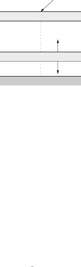
Fig. 6.2 Subdivision of an inhomogeneous atmosphere into N homogeneous sub-
layers. At the boundaries τ
i−1
and τ
i
the up- and downward flux densities are given
by E
+
(τ
i−1
) and E
−
(τ
i
), respectively.
(1) First, solve (6.35) for each individual homogeneous sublayer i defined by the optical
depth interval τ
i
.
(2) The flux densities E
±
(τ
i
) are forced to be continuous at each interior interface τ
i
.
(3) If τ
N
is the total optical depth of the atmosphere then for a reflecting ground the flux
density E
+
(τ
N
) is determined by the diffusely reflected flux density E
−
(τ
N
) plus diffuse
or specular reflection of the direct solar radiation reaching the ground.
(4) Similar to DOM, a linear system of equations has to be solved to obtain the up- and
downward flux densities at each level i of the model atmosphere.
Figure 6.2 illustrates the sublayering of the atmosphere as well as the up- and
downward diffuse flux densities at the boundaries of an arbitrary layer i.
6.3 Different versions of two-stream methods
In this section we will present some two-stream methods which have been widely
discussed in the literature.
6.3.1 Two-stream method with hemispheric isotropy
In this version of TSM it is assumed that the up- and downward diffuse radiation
field is isotropic. Evaluating for this particular situation (6.32) and (6.33) yields
µ
±
= ¯µ =
1
2
, b
±
=
¯
b =
1
0
b(−µ)dµ (6.38)

6.3 Different versions of two-stream methods 167
Truncating in (2.80) the phase function after the linear term, i.e. P(µ, −µ
) =
1 − p
1
µµ
, and substituting this expression into (6.25) results in
b(−µ
) =
1
2
−
3
4
gµ
=⇒
¯
b =
1
2
−
3
8
g (6.39)
Here the so-called asymmetry parameter of the phase function g has been intro-
duced. This quantity is defined by the first moment of the phase function
g =
1
2
1
−1
cos P(cos )d cos =
p
1
3
(6.40)
whereby the integral was evaluated by means of (2.61). Hence it is seen that for
isotropic scattering g = 0.
At this point it is necessary to make a brief remark on the phase function as given
by (2.55). If the phase function is found with the help of the rigorous electromagnetic
theory, known as the Mie–Debye theory to be discussed later, we speak of the Mie
phase function P
Mie
(cos ). Often it is convenient to approximate P
Mie
with the
help of the asymmetry parameter. The resulting phase function is known as the
Henyey–Greenstein phase function defined by
P
HG
(cos ) =
1 − g
2
(1 + g
2
− 2g cos )
3/2
=
∞
l=0
p
l,HG
P
l
(cos )
with p
l,HG
= (2l + 1)g
l
(6.41)
6.3.2 The Eddington approximation
In the classical Eddington approximation the radiance is arranged by means of
I (τ,µ,ϕ) = I
0
(τ ) + µI
1
(τ ) (6.42)
so that I is independent of the azimuthal angle ϕ. Substituting this equation into
(6.21) gives
µ
d
dτ
[
I
0
(τ ) + µI
1
(τ )
]
= I
0
(τ ) + µI
1
(τ ) −
ω
0
2
1
−1
P(µ, µ
)[I
0
(τ ) + µ
I
1
(τ )]dµ
−
ω
0
4π
S
0
exp
−
τ
µ
0
P(µ, −µ
0
) (6.43)

168 Two-stream methods for the solution of the RTE
The multiple scattering integral may be evaluated by means of (2.80) and the
orthogonality relations for the Legendre polynomials (2.59b) yielding
2
1
−1
P(µ, µ
)(I
0
+ µ
I
1
)dµ
= 2I
0
+ 2gµI
1
(6.44)
with g = p
1
/3. Hence, a consequence of the Eddington approximation (6.42) is that
the phase function is truncated after the linear term. Integrating (6.43) over µ in the
limits [−1, 1] we obtain a differential equation for I
1
. Multiplication of (6.43) by
µ and subsequent integration over µ gives the corresponding differential equation
for I
0
. Thus we obtain
dI
1
dτ
= 3(1 − ω
0
)I
0
−
3
4π
ω
0
S
0
exp
−
τ
µ
0
(6.45)
dI
0
dτ
= (1 − ω
0
g)I
1
+
3
4π
ω
0
gµ
0
S
0
exp
−
τ
µ
0
According to (6.22) the up- and downward radiative flux densities are given by
E
+
= π
I
0
+
2
3
I
1
, E
−
= π
I
0
−
2
3
I
1
(6.46)
Hence, I
0
and I
1
may be written as
I
0
=
1
2π
(E
+
+ E
−
), I
1
=
3
4π
(E
+
− E
−
) (6.47)
Substituting these relations into (6.45) we obtain
d
dτ
(E
+
− E
−
) =2(1 −ω
0
)(E
+
+ E
−
) − ω
0
S
0
exp
−
τ
µ
0
(6.48)
d
dτ
(E
+
+ E
−
) =
3
2
(1 − ω
0
g)(E
+
− E
−
) +
3
2
ω
0
gµ
0
S
0
exp
−
τ
µ
0
Addition and subtraction of (6.48a,b) finally results in
d
dτ
E
+
=
(1 − ω
0
) +
3
4
(1 − ω
0
g)
E
+
+
(1 − ω
0
) −
3
4
(1 − ω
0
g)
E
−
−
ω
0
2
1 −
3
2
gµ
0
S
0
exp
−
τ
µ
0
d
dτ
E
−
=−
(1 − ω
0
) −
3
4
(1 − ω
0
g)
E
+
−
(1 − ω
0
) +
3
4
(1 − ω
0
g)
E
−
+
ω
0
2
1 +
3
2
gµ
0
S
0
exp
−
τ
µ
0
(6.49)
2
Recall that P
0
(µ) = 1 and P
1
(µ) = µ.

6.3 Different versions of two-stream methods 169
As stated before, the right-hand side of (6.44) implies a linear approximation of the
phase function so that b(−µ
) and
¯
b are given by (6.39). According to (6.33) the
quantities b
±
are independent of direction. Since
¯
b is also independent of direction,
we approximate b
±
by
¯
b. Assuming additionally that µ
±
= 1/2 we find from (6.37)
and (6.49)
α
11,Ed
= α
11
−
1
4
, α
21,Ed
= α
21
−
1
4
α
12,Ed
= α
11
+
1
4
, α
22,Ed
= α
11
+
1
4
(6.50)
Furthermore, one may easily see that the factors multiplying the solar radiation
terms in (6.49) are given by the components of S as defined in (6.36). The scat-
tering problem based on the approximation (6.42) was treated in some detail
by Shettle and Weinman (1970) and, among others, by Zdunkowski and Junk
(1974).
Two-stream approximations often yield unsatisfactory results because in these
methods the strong forward scattering peak of the phase function is not accounted
for. A distinct improvement of a particular TSM is achieved by utilizing the δ-scaled
phase function defined in (6.1). In the δ-two-stream approach, P
∗
reduces to the
form given in (4.35).
Introducing P
∗
in the classical Eddington method yields the δ-Eddington
approximation where, according to (6.18), the original unscaled parameters
(τ, p
1
,ω
0
) are replaced by (τ
∗
, p
∗
1
,ω
∗
0
) with
τ
∗
= (1 − ω
0
f )τ , p
∗
1
=
p
1
− 3 f
1 − f
, ω
∗
0
=
(1 − f )ω
0
1 − ω
0
f
(6.51)
The fraction f of radiation in the diffraction peak is determined with the help of
(6.9) yielding for n = 2
Mie phase function: f =
p
2
5
Henyey–Greenstein phase function: f =
p
2,HG
5
= g
2
=
p
1
3
2
(6.52)
where in case of the Henyey–Greenstein phase function (6.41) has been used.
Owing to the δ-scaling, the backscattered fraction of the direct solar radiation can
be expressed as
b(−µ
0
) =
1
2
1 −
3
2
g
∗
µ
0
with g
∗
=
g − f
1 − f
=
p
∗
1
3
(6.53)

170 Two-stream methods for the solution of the RTE
6.3.3 Discrete ordinates formalism
Setting in the discrete ordinates method s =1, according to (2.90) the Gaussian
weights and nodes are given by
w
1
= w
−1
= 1, µ
1
=
1
√
3
, µ
−1
=−
1
√
3
(6.54)
Recall that the nodes µ
i
are the positive zeros of the corresponding Legendre
polynomials. Equation (6.54) represents the simplest possible choice for the number
of streams in DOM. The upward and downward radiation streams can be interpreted
as traveling along the directions µ
1
and µ
−1
, respectively. For the backscattered frac-
tion and for a first-order representation of the phase function we obtain from (6.25)
b(−µ
) =
1
2
−
3
2
gµ
1
µ
(6.55)
For the determination of
¯
b equation (6.38) will be evaluated by means of the
Gaussian quadrature. However, it is noteworthy that the double-Gaussian quadra-
ture leading to µ
1
=1/2 is not recommended since for g =1 the quadrature of
1
0
b(−µ
)dµ
yields an unphysical total backscattered fraction
¯
b = 1/8. However,
choosing g =1 means that the total radiation is scattered in the forward direction,
i.e.
¯
b must be zero. With the ordinary Gaussian quadrature one finds indeed the
physically correct value
¯
b =0.
The parameters necessary for evaluating the matrix A in (6.36) are given by
µ
±
= µ
1
= 1/
√
3, b
+
= 1 −
1
2
P(µ
1
,µ
1
), b
−
=
1
2
P(µ
1
, −µ
1
) = b
+
(6.56)
Here the first-order approximation of the phase function
P(µ
1
, ±µ
1
) = 1 ± 3gµ
1
µ
1
= 1 ± g (6.57)
has been used. In the primary scattering term the phase function and the correspond-
ing backscattered fraction for the primary scattered sunlight are approximated as
P(µ
0
, ±µ
1
) = 1 ±
√
3gµ
0
=⇒ b(−µ
0
) =
1
2
P(µ
0
, −µ
1
) =
1
2
1 −
√
3gµ
0
(6.58)
6.3.4 Practical improved flux method
In the so-called practical improved flux method (PIFM) by Zdunkowski et al. (1982)
the following parameters are employed
µ
±
= ¯µ =
1
2
, b
±
=
¯
b =
3
8
(1 − g), b(−µ
0
) =
1
2
−
3
4
gµ
0
(6.59)

6.3 Different versions of two-stream methods 171
It is to be noted that in PIFM the δ-scaling of the phase function is applied to the
primary scattering term only, that is
d
dτ
E
+
prim
= ω
0
(1 − f )b
∗
(−µ
0
)S
0
exp
−
(1 − ω
0
f )τ
µ
0
d
dτ
E
−
prim
= ω
0
(1 − f )[1 − b
∗
(−µ
0
)]S
0
exp
−
(1 − ω
0
f )τ
µ
0
(6.60)
The δ-scaled backscattered fraction for primary scattered light is defined by
b
∗
(−µ
0
) =
1
2
−
3
4
g
∗
µ
0
=
1
2
−
3
4
g − f
1 − f
µ
0
(6.61)
The particular choices (6.60) replace the primary scattering term on the right-hand
side of (6.35). In PIFM the transfer of the diffuse radiation still employs the unscaled
optical parameters ω
0
and b. For PIFM the coefficients of the matrix A are then
given by
α
11
=−α
22
=
1 − ω
0
(1 −
¯
b)
¯µ
, α
12
=−α
21
=−
ω
0
¯
b
¯µ
(6.62)
This selective type of scaling prevents negative flux densities which occasionally
occur in case of the traditional δ-scaling.
Finally, we will state different advantages and disadvantages of the two-stream
methods.
(1) Two-stream methods are computationally very fast and can be employed as a standard
technique for radiative transfer calculations in climate models.
(2) It is easy to apply modifications to a particular TSM which account for partial cloudi-
ness. Details will be given in Section 5.6 of this chapter.
(3) Two-stream methods yield sufficiently accurate results for radiative heating and cooling
rates. Maximum errors are typically in the order of 10%.
(4) Application of the δ-scaled phase function yields distinct improvements of the results
of the corresponding δ-two-stream methods.
The derivation of the TSM as outlined above follows mainly the work of
Zdunkowski et al. (1980), Zdunkowski and Korb (1985), and Ceballos (1988).
However, many more versions of TSMs (see, e.g. Meador and Weaver, 1980; Bott
and Zdunkowski, 1983) can be found in the literature which all have their particular
advantages and disadvantages.

172 Two-stream methods for the solution of the RTE
6.4 Analytical solution of the two-stream methods
for a homogeneous layer
In all versions of TSM presented in the previous section it turned out that µ
+
= µ
−
and b
+
= b
−
. In this case the coefficients of the matrix A are related by α
11
=−α
22
and α
21
=−α
12
, see (6.37), and the RTE (6.35) reduces to
dE
+
dτ
dE
−
dτ
=
α
1
− α
2
α
2
− α
1
E
+
E
−
+
α
3
α
4
S (6.63)
Here the abbreviations
α
1
= α
11
, α
2
= α
21
, α
3
=−ω
0
b(−µ
0
), α
4
= ω
0
[
1 − b(−µ
0
)
]
(6.64)
have been introduced while the solar radiation S(τ ) is given by the solution of the
differential equation
dS
dτ
=−
1
µ
0
S
0
exp
−
τ
µ
0
=⇒ S(τ ) = S
0
exp
−
τ
µ
0
(6.65)
Equation (6.63) describes a set of coupled ordinary differential equations for E
+
and E
−
. For a homogeneous layer τ
i
= τ
i
− τ
i−1
the coefficients α
j
, j = 1,...,4
of the system are constant so that it is possible to obtain analytical solutions. First
we solve the homogeneous system
dE
+
dτ
dE
−
dτ
=
α
1
−α
2
α
2
−α
1
E
+
E
−
(6.66)
Inserting the trial solutions E
+
= A
1
exp(
˜
λτ ), E
−
= A
2
exp(
˜
λτ ) into (6.66) yields
the linear equation
α
1
−
˜
λ −α
2
α
2
−α
1
−
˜
λ
E
+
E
−
= 0 (6.67)
This equation can be fulfilled only if the determinant vanishes, i.e.
α
1
−
˜
λ −α
2
α
2
−α
1
−
˜
λ
=−(α
1
−
˜
λ)(α
1
+
˜
λ) + α
2
2
= 0 (6.68)

6.4 Analytical solution of TSMs for a homogeneous layer 173
From (6.68) we obtain the two eigenvalues of the system
˜
λ
1,2
=±λ with λ =
$
α
2
1
− α
2
2
(6.69)
A solution of the homogeneous system can be obtained by inserting the expressions
˜
λ
1
: E
+
= C
1
exp
(
λτ
)
, E
−
= D
1
exp
(
λτ
)
˜
λ
2
: E
+
= C
2
exp
(
−λτ
)
, E
−
= D
2
exp
(
−λτ
)
(6.70)
into (6.67) yielding
˜
λ
1
:(α
1
− λ)C
1
− α
2
D
1
= 0,α
2
C
1
− (α
1
+ λ)D
1
= 0
˜
λ
2
:(α
1
+ λ)C
2
− α
2
D
2
= 0,α
2
C
2
− (α
1
− λ)D
2
= 0
(6.71)
From these equations the ratio of the constants can be determined as
D
1
=
(α
1
− λ)
α
2
C
1
=
α
2
(α
1
+ λ)
C
1
D
2
=
(α
1
+ λ)
α
2
C
2
=
α
2
(α
1
− λ)
C
2
(6.72)
with
α
2
(α
1
+ λ)
=
(α
1
− λ)
α
2
(6.73)
which is equivalent to λ =
$
α
2
1
−α
2
2
. The general solution of the homogeneous
system, including two constants of integration, is given by a superposition of the
individual solutions and may be written as
E
+, h
(τ ) = C
1
exp(λτ) +C
2
exp(−λτ)
E
−, h
(τ ) = C
1
α
2
(α
1
+ λ)
exp(λτ) +C
2
α
2
(α
1
− λ)
exp(−λτ)
(6.74)
In the next step we determine a particular solution of the inhomogeneous system.
This can be most easily obtained by using a trial solution having the functional form
of the inhomogeneous term of the differential equation (6.63), that is
E
+, p
(τ ) = α
5
S
0
exp
−
τ
µ
0
, E
−, p
(τ )= α
6
S
0
exp
−
τ
µ
0
(6.75)
Inserting these trial solutions into the inhomogeneous system (6.63) leads to another
inhomogeneous system of linear equations for α
5
and α
6
1
µ
0
+ α
1
−α
2
α
2
1
µ
0
− α
1
α
5
α
6
+
α
3
α
4
= 0 (6.76)

174 Two-stream methods for the solution of the RTE
with the solutions
α
5
=
α
1
−
1
µ
0
α
3
− α
2
α
4
1
µ
0
2
− λ
2
, α
6
=
α
2
α
3
−
α
1
+
1
µ
0
α
4
1
µ
0
2
− λ
2
(6.77)
Inspection of these equations reveals that for µ
0
=1/λ the constants α
5
and α
6
become infinitely large. However, this so-called resonance case may be easily
avoided by adding to the actual solar position µ
0
a small increment ±µ
0
.
In the third step, the complete solution of the inhomogeneous system of lin-
ear differential equations (6.63) is obtained by adding the homogeneous and the
particular solutions (6.74) and (6.75). Hence we obtain
E
+
(τ ) = C
1
exp(λτ) +C
2
exp(−λτ) + α
5
S
0
exp
−
τ
µ
0
E
−
(τ ) = C
1
α
2
(α
1
+ λ)
exp(λτ) +C
2
α
2
(α
1
− λ)
exp(−λτ) + α
6
S
0
exp
−
τ
µ
0
(6.78)
Our final goal is to obtain expressions for the flux densities E
+
(τ
i−1
) and E
−
(τ
i
)
leaving the homogeneous layer τ
i
in terms of the flux densities E
−
(τ
i−1
) and
E
+
(τ
i
) entering this layer. With the help of (6.78), the incident flux densities at the
boundaries of the layer can be written down immediately
E
+
(τ
i
) = C
1
exp(λτ
i
) + C
2
exp(−λτ
i
) + α
5
S(τ
i−1
)exp
−
τ
i
µ
0
E
−
(τ
i−1
) = C
1
α
2
(α
1
+ λ)
exp(λτ
i−1
) + C
2
α
2
(α
1
− λ)
exp(−λτ
i−1
) + α
6
S(τ
i−1
)
(6.79)
where S(τ
i−1
) is the solar radiative flux density incident at the top of the layer, that
is
S(τ
i−1
) = S
0
exp
−
τ
i−1
µ
0
(6.80)
Equations (6.79) may be solved to determine the integration constants C
1
and
C
2
. The result is
C
1
= β
11
E
+
(τ
i
) + β
12
E
−
(τ
i−1
) + β
13
S(τ
i−1
)
C
2
= β
21
E
+
(τ
i
) + β
22
E
−
(τ
i−1
) + β
23
S(τ
i−1
)
(6.81)