Zdunkowski W., Trautmann T., Bott A. Radiation in the atmosphere: A course in Theoretical Meteorology
Подождите немного. Документ загружается.


5.1 Adjoint formulation of the RTE 135
Now we will derive the adjoint formulation of the transfer problem as well as
the proper boundary conditions. The theory of linear operators defines the adjoint
linear differential operator L
+
corresponding to the linear differential operator L.
The operator L
+
is uniquely defined if for any two arbitrary functions I and I
+
the
following relation is valid
I
+
, LI=L
+
I
+
, I or LI, I
+
=I, L
+
I
+
(5.7)
The validity of the second equation, that is the possibility to interchange the expres-
sions within a bracket, follows immediately from the definition of the inner product
(5.6). In radiative transfer problems the two functions I and I
+
represent the radi-
ance and the adjoint radiance, respectively.
Now the problem arises in which way L
+
should be determined. This could
be done by imposing suitable boundary conditions on I
+
and then attempt to
derive L
+
. Simple examples of this type are given by Friedman (1956) and Keener
(1988). At this point we recommend that the student consults Appendix 5.5.1 to this
chapter. It might be more practical, however, to follow Bell and Glasstone (1970) by
postulating L
+
and then determine the appropriate boundary conditions on I
+
. Box
et al. (1988) successfully used the second type of approach. Their approach will be
described in this chapter. It appears that Gerstl (1982) introduced the adjoint method
into the meteorological literature on radiative transfer. The adjoint formulation to
solve transport problems was also successfully applied in reactor physics.
We will now introduce the adjoint linear differential operator L
+
by means of
L
+
=−µ
∂
∂z
+ k
ext
(z) −
k
sca
(z)
4π
4π
P(z, Ω → Ω
) ◦ d
(5.8)
which differs from (5.5) only in the sign of the first term, also known as the streaming
term, and the interchange of the initial and final directions Ω and Ω
in the phase
function. According to the discussion in Section 1.6.2 for homogeneous spherical
particles the scattering process depends only on the cosine of the scattering angle
cos = Ω
· Ω, see (1.43). Since the commutative law holds for the scalar product
of two vectors we may write
P(z, Ω
→ Ω) = P(z, Ω
· Ω) = P(z, Ω · Ω
) = P(z, Ω → Ω
) (5.9)
so that the only real difference between L and L
+
is the opposite sign of the
streaming term.
In analogy to the forward form (5.5) of the RTE, the adjoint form of the radiative
transfer equation can be written as
L
+
I
+
(z, Ω) = Q
+
(z, Ω)
(5.10)

136 Radiative perturbation theory
At this point the adjoint source Q
+
will be left completely unspecified. For mathe-
matical convenience and also for purposes of interpretation, we introduce a function
(z, Ω) according to the definition
(z, Ω) = I
+
(z, −Ω) (5.11)
Inserting this definition into (5.10), using L
+
as defined by (5.8), results in
Q
+
(z, Ω) =
−µ
∂
∂z
+ k
ext
(z)
(z, −Ω) −
k
sca
(z)
4π
×
4π
P(z, Ω → Ω
)(z, −Ω
)d
(5.12)
In order to transform this operator equation to the form (5.5), we use the substitutions
Ω →−Ω and Ω
→−Ω
. Since Ω = Ω(µ, ϕ) and ϕ ≥ 0, it is obvious that the
change of sign of the direction vector Ω also requires a change of sign of µ so that
instead of (5.12) we obtain
Q
+
(z, −Ω) =
µ
∂
∂z
+ k
ext
(z)
(z, Ω)−
k
sca
(z)
4π
×
4π
P(z, −Ω →−Ω
)(z, Ω
)d
(5.13)
According to (5.9) we may write
P(z, −Ω →−Ω
) = P(z, Ω → Ω
) = P(z, Ω
→ Ω) = P(z, Ω
· Ω) (5.14)
Utilizing this information together with (5.13) in (5.10) yields for the adjoint form
of the RTE
L(z, Ω) = Q
+
(z, −Ω)
(5.15)
This form involves the linear differential operator L, the function (z, Ω) and the
adjoint source Q
+
for the direction −Ω. The term is also called the pseudo-
radiance.
We will now briefly summarize the previous discussion by momentarily assum-
ing that the adjoint source Q
+
is known.
(i) In order to determine the radiance I
+
(z, Ω) due to the adjoint source Q
+
(z, Ω), we
first solve the forward RTE (5.15) for the pseudo-source Q
+
(z, −Ω). This yields the
auxiliary function (z, Ω).
(ii) Changing the direction according to (5.11) results in the adjoint radiance I
+
(z, Ω).
(iii) For the determination of the auxiliary function , any standard solution method can be
used to solve the RTE (5.15). Certainly, the accuracy of the adjoint radiance calculations
equals the accuracy of the chosen forward procedure.

5.2 Boundary conditions 137
5.2 Boundary conditions
With the help of physical arguments it is a rather simple matter to specify the
boundary conditions for the radiance I . It is much more difficult, in the general case,
to obtain the boundary conditions for the adjoint radiance I
+
which is not readily
visualized. It might be preferable to think of the function I
+
as a mathematical entity
which was introduced for operational purposes and less on grounds of physical
arguments. In order to obtain the boundary conditions for the adjoint radiances I
+
we apply the definition (5.7) and obtain
z
t
0
4π
I
+
(z, Ω)
µ
∂
∂z
I (z, Ω) + k
ext
(z)I (z, Ω)
−
k
sca
(z)
4π
P(z, Ω
→ Ω)I (z, Ω
)d
d dz
=
z
t
0
4π
I (z, Ω)
−µ
∂
∂z
I
+
(z, Ω) +k
ext
(z)I
+
(z, Ω)
−
k
sca
(z)
4π
4π
P(z, Ω → Ω
)I
+
(z, Ω
)d
d dz
(5.16)
As will be observed, we have two sets of functions. The first set contains the
radiances I (z, Ω) to which we apply the operator L and certain boundary conditions
to be specified shortly. The second set consists of the adjoint radiances I
+
to which
we apply the operator L
+
and some boundary conditions which may differ from
the boundary conditions that apply to the radiances I .
Obviously, the second terms on each side of (5.16) drop out. After renaming the
integration variables, we find that the third terms also cancel so that we obtain
z
t
0
4π
µI
+
(z, Ω)
∂
∂z
I (z, Ω)d dz =−
z
t
0
4π
µ
∂
∂z
I
+
(z, Ω)I (z, Ω)d dz
(5.17)
Performing a partial integration of the right-hand side of (5.17) over z from z = 0
to z = z
t
we obtain
z
t
0
4π
µI
+
(z, Ω)
∂
∂z
I (z, Ω)d dz =−
4π
µI
+
(z, Ω)I (z, Ω)d
z=z
t
z=0
+
z
t
0
4π
µI
+
(z, Ω)
∂
∂z
I (z, Ω)d dz
(5.18)
from which follows immediately
4π
µI
+
(z
t
, Ω)I (z
t
, Ω)d =
4π
µI
+
(0, Ω)I (0, Ω)d (5.19)

138 Radiative perturbation theory
The evaluation of this equation requires the specification of the boundary conditions
for I and I
+
.
5.2.1 Vacuum boundary conditions
The vacuum boundary conditions for the radiance I state that an atmospheric layer
is illuminated only by the parallel radiation of the Sun while diffuse illumination
at the boundaries of the layer is not admitted. Since at the top of the atmosphere
the incoming parallel solar radiation is already included in the source term Q,it
does not have to be considered here. Thus, the vacuum boundary conditions can be
stated in the form
top of the atmosphere: I(z
t
,µ,ϕ) = 0, 0 ≤ ϕ ≤ 2π, −1 ≤ µ<0
Earth’s surface: I (0,µ,ϕ) = 0, 0 ≤ ϕ ≤ 2π,0<µ≤ 1
(5.20)
In order to apply these equations, we split (5.19) as shown into
2π
0
0
−1
µI
+
(z
t
,µ,ϕ)I (z
t
,µ,ϕ)dµdϕ +
2π
0
1
0
µI
+
(z
t
,µ,ϕ)I (z
t
,µ,ϕ)dµdϕ
=
2π
0
0
−1
µI
+
(0,µ,ϕ)I (0,µ,ϕ)dµdϕ
+
2π
0
1
0
µI
+
(0,µ,ϕ)I (0,µ,ϕ)dµdϕ
(5.21)
Thus, with the help of (5.20), we recognize immediately that (5.21) reduces to
2π
0
1
0
µI
+
(z
t
,µ,ϕ)I (z
t
,µ,ϕ)dµdϕ =
2π
0
0
−1
µI
+
(0,µ,ϕ)I (0,µ,ϕ)dµdϕ
(5.22)
We note that the radiances I and I
+
appearing in this equation are completely
arbitrary and independent of each other. In the range of integration the radiances
I (z
t
,µ,ϕ) and I (0,µ,ϕ) differ from zero. Thus, the only way to satisfy (5.22) is
to require that the boundary conditions of the adjoint radiances are given by
top of the atmosphere: I
+
(z
t
,µ,ϕ) = 0, 0 ≤ ϕ ≤ 2π,0<µ≤ 1
Earth’s surface: I
+
(0,µ,ϕ) = 0, 0 ≤ ϕ ≤ 2π, −1 ≤ µ<0
(5.23)
Summarizing, the vacuum boundary conditions of the regular radiances I require
that the incoming diffuse radiation is zero at the base and the top of the atmosphere
while in the adjoint formulation the outgoing radiances I
+
at the boundaries must be
zero. We refer to the solution of the RTE utilizing the vacuum boundary conditions
as the standard problem. For further reference see also Chapter 3.

5.2 Boundary conditions 139
5.2.2 Boundary conditions for a reflecting surface
The most important extension of the standard problem is the inclusion of ground
reflection. For simplicity, we will assume a Lambertian surface with albedo A
g
.As
already mentioned previously, such a surface reflects the incoming radiances from
the upper hemisphere isotropically according to
π I (0,µ,ϕ) = A
g
2π
0
0
−1
|µ
|I (0,µ
,ϕ
)dµ
dϕ
,0<ϕ≤ 2π ,0<µ≤ 1
(5.24)
Since the integration is over all directions, the right-hand side of this equation is
independent of any direction so that the upward radiance I (0,µ,ϕ) must also be
independent of direction, that is it has the same value for every of µ and ϕ.
The inclusion of the surface reflection also requires a change of the lower
adjoint boundary conditions in (5.23) while the upper adjoint boundary condi-
tion in (5.23) remains unaffected. Let us return to equation (5.21). Substituting
the upper boundary conditions of (5.20) and (5.23) into (5.21) we find that the
left-hand side vanishes. Substitution of (5.24) into the right-hand side of (5.21)
yields
2π
0
0
−1
µI
+
(0,µ,ϕ)I (0,µ,ϕ)dµdϕ
=−
A
g
π
2π
0
0
−1
|µ
|I (0,µ
,ϕ
)dµ
dϕ
2π
0
1
0
µI
+
(0,µ,ϕ)dµdϕ
=
A
g
π
2π
0
0
−1
µI (0,µ,ϕ)dµdϕ
2π
0
1
0
µ
I
+
(0,µ
,ϕ
)dµ
dϕ
(5.25)
In the integral on the left-hand side only the function I
+
(0,µ,ϕ), (−1 ≤ µ<0),
is unknown. Since I and I
+
are independent of each other, we conclude that in this
integral I
+
(0,µ,ϕ) must be given by the following expression
π I
+
(0,µ,ϕ) = A
g
2π
0
1
0
µ
I
+
(0,µ
,ϕ
)dµ
dϕ
,0<ϕ≤ 2π , − 1 ≤ µ<0
(5.26)
By comparing this equation with (5.24) the symmetry between the forward and
the adjoint boundary conditions becomes apparent. More complicated boundary
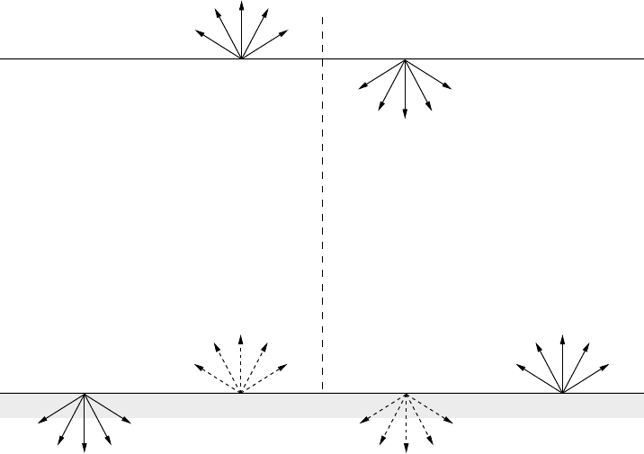
formulations are possible but will not be considered here. Figure 5.1 depicts some
information about the forward and the adjoint formulation showing the various
directions of the regular and the adjoint radiances at the upper and lower boundary
of the atmosphere.
140 Radiative perturbation theory
µ<0 µ>0 µ<0 µ>0
I(z
t
, µ, ϕ)=0
I(0, µ, ϕ)
I
+
(0, µ, ϕ)
I(z
t
, µ, ϕ)= 0
I
+
(
z
t
, µ, ϕ)= 0
I
+
(
z
t
, µ, ϕ)=0
= 0
I(0, µ
=0
= 0
=0
= 0
Forward method Adjoint method
z = z
t
z =0
{
I
+
(
0
, µ, ϕ)
{
/
, ϕ)= 0
/
/
/
/
/
Fig. 5.1 Comparison of directions of radiances in the forward and the adjoint
formulation. Dashed arrows indicate no reflection (... = 0) or reflection at the
Earth’s surface (... = 0).
5.2.3 Inclusion of surface reflection in the formulation of the radiances
Equation (5.26) gives the ground reflection in the adjoint formulation. Now we must
find a general expression for the adjoint radiance in the presence of ground reflection
which applies to an arbitrary height. This task will be accomplished by first finding
a suitable expression in the forward mode which can then be transformed to the
adjoint formulation.
Let I
v
(z,µ,ϕ) represent the solution of the standard problem, that is the solution
of the RTE with vacuum boundary conditions (index v) and source term Q
LI
v
(z,µ,ϕ) = Q(z,µ,ϕ) (5.27)
Then the downward flux density in the forward mode at the Earth’s surface (z = 0)
is given by
E
v,−
(0) =
2π
0
0
−1
|µ|I
v
(0,µ,ϕ)dµdϕ (5.28)

5.2 Boundary conditions 141
For purely mathematical purposes, in analogy to the form (5.3), we introduce an
artificial surface source Q
g
by means of
Q
g
=
µδ(z)0<µ≤ 1
0 −1 ≤ µ<0
(5.29)
Now let I
g
(z,µ,ϕ) represent the solution of the RTE with vacuum boundary
conditions and source term Q
g
LI
g
(z,µ,ϕ) = Q
g
(z,µ,ϕ) (5.30)
Owing to the special formulation of the surface source Q
g
the radiance I
g
is a
dimensionless quantity.
2
The corresponding dimensionless downward flux density
E
g,−
(0) at the surface is given by
E
g,−
(0) =
2π
0
0
−1
|µ|I
g
(0,µ,ϕ)dµdϕ (5.31)
In Appendix 5.5.2 we will show that I (z,µ,ϕ) may be written as function of the
vacuum solution and the solution with surface reflection in the form
I (z,µ,ϕ) = I
v
(z,µ,ϕ) + E
v,−
(0)
A
g
π
1 −
A
g
π
E
g,−
(0)
I
g
(z,µ,ϕ) (5.32)
This expression shows in which way at an arbitrary height z the radiance I (z,µ,ϕ)
is influenced by the ground albedo A
g
.
The task ahead is to transform equation (5.32) to the adjoint representation.
To this end we first consider the vacuum problem without any surface reflection.
By repeating (5.10), adding the suffix v to I
+
(vacuum boundary conditions) for
distinction, we obtain
L
+
I
+
v
(z,µ,ϕ) = Q
+
(z,µ,ϕ) (5.33)
Using (5.11), we find the auxiliary function for the vacuum problem
v
(z,µ,ϕ) = I
+
v
(z, −µ, ϕ) (5.34)
According to (5.15), the auxiliary function
v
satisfies the forward RTE with source
Q
+
(z, −µ, ϕ)
L
v
(z,µ,ϕ) = Q
+
(z, −µ, ϕ) (5.35)
2
Note that the unit of δ(z)is(m
−1
).
142 Radiative perturbation theory
The vacuum boundary conditions for
v
may be obtained by substituting (5.34)
into (5.23).
For the reflecting surface we obtain from (5.26)
π(0,−µ, ϕ) = A
g
2π
0
1
0
µ
(0, −µ
,ϕ
)dµ
dϕ
, 0<ϕ≤ 2π, −1 ≤ µ< 0
(5.36)
which may also be written as
π(0,µ,ϕ) = A
g
2π
0
0
−1
|µ
|(0,µ
,ϕ
)dµ
dϕ
, 0 <ϕ≤ 2π, 0 <µ≤ 1
(5.37)
To include the surface reflection in the adjoint formulation we may proceed
analogously to the forward formulation. Comparison of (5.35) with (5.5) shows
that the auxiliary function
v
(z,µ,ϕ) enters the RTE in the same way as the
forward radiance I (z,µ,ϕ) if the source Q(z,µ,ϕ) is replaced by Q
+
(z, −µ, ϕ).
Furthermore, comparison of equation (5.37) with (5.24) shows the direct analogy of
the lower boundary conditions of (0,µ,ϕ) and I (0,µ,ϕ). These two comparisons
imply that the auxiliary function describing the radiation field including ground
reflection should be given by an expression which is analogous to the form (5.32),
that is
(z,µ,ϕ) =
v
(z,µ,ϕ) +
˜
E
v,−
(0)
A
g
π
1 −
A
g
π
˜
E
g,−
(0)
g
(z,µ,ϕ) (5.38)
where the terms
˜
E
v,−
(0) and
˜
E
g,−
(0) are still unspecified. The quantity
g
(z,µ,ϕ)
is the solution to
L
g
(z,µ,ϕ) = Q
g
(z,µ,ϕ) (5.39)
with vacuum boundary conditions for
g
, and Q
g
as defined by (5.29).
We are now able to find the meanings of
˜
E
v,−
(0) and
˜
E
g,−
(0). Comparison of
(5.39) with (5.30), observing (5.11), yields the following identities:
I
g
(z,µ,ϕ) =
g
(z,µ,ϕ) = I
+
g
(z, −µ, ϕ) (5.40)
According to (5.31) and due to the similarities of the forms stated by (5.32) and
(5.38), for the quantity
˜
E
g,−
(0) we conjecture
˜
E
g,−
(0) =
2π
0
0
−1
|µ|
g
(0,µ,ϕ)dµdϕ = E
g,−
(0) (5.41)

5.3 Radiative effects 143
The form of
˜
E
v,−
(0) follows from (5.28) so that
˜
E
v,−
(0) =
2π
0
0
−1
|µ|
v
(0,µ,ϕ)dµdϕ =
2π
0
1
0
µI
+
v
(0,µ,ϕ)dµdϕ = E
+
v,−
(0)
(5.42)
Moreover, from (5.34) we find
v
(z, −µ, ϕ) = I
+
v
(z,µ,ϕ) (5.43)
Utilizing these pieces of information, we are ready to write down the desired adjoint
relationship to handle surface reflection
I
+
(z,µ,ϕ) = I
+
v
(z,µ,ϕ) + E
+
v,−
(0)
A
g
π
1 −
A
g
π
E
g,−
(0)
I
g
(z, −µ, ϕ) (5.44)
Admittedly, some of the above arguments are somewhat indirect.
In order to solve the forward as well as the adjoint problem, including ground
reflection, we have to treat three individual problems:
(i) solution of LI
v
= Q
(ii) solution of LI
g
= Q
g
(iii) solution of L
+
I
+
v
= Q
+
.
It should be noted that the solution for I
g
plays a dual role since it is needed to
solve the forward problem (5.32) as well as the adjoint problem (5.44).
5.3 Radiative effects
Many practical applications do not require the complete information contained
in the radiation field which is described by the distribution of the radiances at a
particular point. Often it is sufficient to extract certain integral quantities from the
field such as upward and downward flux densities, net flux densities at certain
heights and radiative heating rates in selected atmospheric layers. Each integral
quantity is known as the radiative effect E.
The reader will have noticed that the adjoint method was introduced without any
particular motivation. We will now give a convincing reason why this method was
introduced and point out the enormous advantage this method offers when solving
certain radiative transfer problems.
In case of the forward mode, the radiance I follows from the solution of the RTE
LI = Q (5.45)

144 Radiative perturbation theory
The radiative effect E of the radiation field is expressed by the general definition
E = < R, I > (5.46)
where R(z,µ,ϕ) is known as the corresponding response function. To state it more
clearly: to each radiative effect belongs a response function R which expresses the
response of the medium to the illumination of the atmosphere by the source Q.
Soon we will give examples of how to formulate R.
Now we briefly consider the RTE of the corresponding adjoint problem
L
+
I
+
= Q
+
(5.47)
We recall that the adjoint source Q
+
was not specified previously. Since Q
+
is
completely arbitrary we are free to set Q
+
= R. This particular choice of Q
+
results in the advantages of the adjoint method that we have mentioned above.
Combining (5.46) and (5.47) with R = Q
+
we obtain
E =R, I =Q
+
, I =L
+
I
+
, I =I
+
, LI=I
+
, Q
(5.48)
where the last two expressions have been obtained by means of (5.7) and (5.45).
To familiarize ourselves with the formulation of the response function, we con-
sider a few very useful examples.
Example I
Suppose, at level z
0
we wish to calculate the downward flux density E
−
(z
0
) which
is a typical effect of the radiation field. The basic formula is
E = E
−
(z
0
) =
2π
0
0
−1
|µ|I (z
0
,µ,ϕ)dµdϕ (5.49)
In order to state R, we make use of the Heaviside step function U, defined by
U (x − a) =
1 x > a
0 x < a
(5.50)
Utilizing (5.50) equation (5.49) can also be expressed as
E =
z
t
0
2π
0
1
−1
|µ|δ(z − z
0
)U(−µ)I (z,µ,ϕ)dµ dϕ dz
=|µ|δ(z − z
0
)U(−µ), I
(5.51)
Comparison of this equation with (5.46) shows that the response function R is given
by
R(z,µ) =|µ|δ(z − z
0
)U(−µ) (5.52)