Zdunkowski W., Trautmann T., Bott A. Radiation in the atmosphere: A course in Theoretical Meteorology

Подождите немного. Документ загружается.

5.3 Radiative effects 145

U(zz

)

U(z

U(zz

)U(z

−

−−

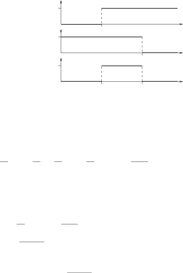
Fig. 5.2 Arrangement of the Heaviside step functions U (z − z

), U (z

− z) and

the product U(z − z

)U(z

− z).

Example II

Suppose we wish to ﬁnd the average spectral solar heating rate within an atmo-

spheric layer z = z

− z

. Omitting in (2.46) the thermal emission J

we integrate

this equation over z yielding

∂T

∂t



rad,z

z



∂T

∂t



rad

dz =

z



2π



−1

abs

(z)

ρ(z)c

I (z,µ,ϕ)dµ dϕ

(5.53)

In order to ﬁnd the response function R, we use the product of two Heaviside step

functions U (z − z

)U(z

− z), see Figure 5.2. Thus for this particular example the

radiative effect E representing the radiative temperature change of layer z is given

E =

z



2π



−1

abs

(z)

ρ(z)c

U (z − z

)U(z

− z)I (z,µ,ϕ)dµ dϕ

abs

(z)

ρ(z)c

z

U (z − z

)U(z

− z), I

(5.54)

yielding the response function as

R(z) =

abs

(z)

ρ(z)c

z

U (z − z

)U(z

− z) (5.55)

Example III

From (5.48) we see that there exist two ways of computing the radiative effect E.

The ﬁrst is the standard or the forward approach. We solve the RTE assuming the

146 Radiative perturbation theory

presence of the source Q, and then we take the inner product of the solution I

with the response function R. The second approach is to solve the adjoint form of

the RTE with source Q

= R, and then take the inner product of the solution I

with the forward source Q. Which one of these two approaches is to be preferred?

If one is interested to compute a single radiative effect, corresponding to a single

source Q, then it does not matter which method is given preference. However, if we

wish to compute the radiative effect of a whole series of sources then one should

choose very judiciously. In the following example, we will demonstrate which type

of method offers the greatest numerical advantage.

Suppose we wish to calculate the downward ﬂux density arriving at the Earth’s

surface. The basic formula is given by setting z

= 0 in (5.49) or in the response

function (5.52). The radiance I (0,µ,ϕ) is found by solving the forward form of

the RTE (5.45) utilizing the source distribution function (5.3). However, the same

radiative effect can be found from (5.48), or explicitly

E =I

, Q=



2π



−1

(z,µ,ϕ)Q(z,µ,ϕ)dµ dϕ dz (5.56)

Inserting here for Q(z,µ,ϕ) the expression (5.3) the integration can be performed

analytically and we obtain

E = E

−

(0) =|µ

,µ

,ϕ

) (5.57)

This interesting result shows that the downward ﬂux density at the ground is com-

pletely determined by the adjoint radiance I

at the top of the atmosphere at z

for

the special direction (µ

,ϕ

). Moreover, the source ﬂux density is |µ

where

is the solar constant for the particular wavelength under consideration. For a

broader solar band an integration over the wave number or the wavelength needs

to be carried out.

Let us reconsider the classical solution (5.49) to ﬁnd E

−

(0). For each given

direction (µ

,ϕ

) of the Sun, i.e. for a ﬁxed Q, the forward RTE (5.45) must be

solved to ﬁnd the corresponding distribution I (0,µ,ϕ). If the daily course of the

downward directed radiative ﬂux density at the ground is required on the basis of

N solar positions, the RTE (5.45) must be solved N times, that is for each position

(µ

,ϕ

) of the Sun.

If we employ the adjoint formulation, we must solve (5.47), choosing as the

adjoint source Q

= R. In practice, the adjoint radiance distribution at the top of

the atmosphere, I

,µ,ϕ), is calculated for all directions (µ, ϕ). This includes

all solar angles (µ

,ϕ

). Thus, plotting the values |µ

,µ

,ϕ

) versus µ

gives the diurnal course of E

−

(0) for all µ

. In one-dimensional slab geometry,

E as well as I

are invariant to ϕ

. Hence only one single adjoint solution of the

RTE is required in comparison to N necessary forward computations. This is the

decisive advantage that the adjoint method offers for many interesting situations.

5.4 Perturbation theory for radiative effects 147

Additional information concerning the advantage of the adjoint formulation of the

RTE can be found in Gerstl and Zardecki (1985).

5.4 Perturbation theory for radiative effects

As is well-known, the calculation of radiative effects for realistic scattering and

absorbing atmospheres requires a large computer effort if exact solutions of the RTE

are demanded. In contrast, the use of approximate methods reduces the computer

effort substantially. The amount of accuracy which is lost due to approximation

depends on the type of the chosen approach. As a ﬁrst approximation method, we

now introduce the so-called perturbation theory which greatly differs from all the

other approximation procedures to be discussed in the next chapter. A number of

more or less successful attempts in this direction have been made to treat aerosol

scattering as a perturbation applied to a Rayleigh scattering atmosphere of ﬁxed

optical path length, see e.g. Sekera (1956), Deirmendjian (1957, 1959) and Box and

Deepak (1979). A different approach is due to Fymat and Abhyankar (1969a,b) and

Abhyankar and Fymat (1970a,b) who considered variations of the single scattering

albedo as a perturbation to simulate aerosol scattering.

In this section we are going to introduce still another procedure due to Box et al.

(1989a) which is a natural continuation of the theoretical developments described

in the previous sections. The main idea is to ﬁrst solve the RTE for a certain

realistic base atmosphere. Solutions to ‘neighboring’ atmospheres can be obtained

by perturbing the functions characterizing the base atmosphere. Since the radiative

transport operator L is not self-adjoint, i.e. L = L

, not only the forward radiance,

but also the adjoint radiance will have to be accounted for. This method is not only

fast but in most cases also quite accurate. It has also been shown that this type

of the perturbation technique can be further developed to improve the accuracy

of the procedure without losing a substantial amount of the numerical advantages

characterizing the present stage of development.

Before we begin with the discussion of the perturbation technique, we would

like to convince the reader that the following treatment is not simply an academic

exercise. Often it is wrongly argued that with the development of ever faster com-

puters, all approximation methods will soon be entirely obsolete. It should not be

overlooked that with the advent of faster computers more realistic and thus more

complex weather forecasting and climate prediction models are being developed

which require the implementation of increasingly more accurate and still faster

radiation transfer codes. Since the exact and frequent evaluation of the RTE for the

entire spectrum is out of the question for some time to come, the development of

improved approximation methods is a matter of necessity. The perturbation tech-

nique has the potential of being such a method. Thus we are not simply presenting

an academic exercise but a procedure of great usefulness.

148 Radiative perturbation theory

5.4.1 Basic perturbation theory

The state of the atmosphere is characterized by functions such as k

ext

(z), k

sca

(z)

and P(z, Ω). We must distinguish between the operators, the radiances and func-

tions of the perturbed atmosphere and the corresponding quantities describing the

base atmosphere. This will be done by attaching a zero as subscript to all sym-

bols characterizing the base atmosphere. Thus, instead of (5.4), (5.8), (5.45) and

(5.47) henceforth denoting the equations for the perturbed atmosphere, for the base

atmosphere we write

(a) L

(z, Ω) = Q, (b) L

(z, Ω) = Q

= R

(5.58)

with

(a) L

= µ

∂

∂z

+ k

ext,0

(z) −

sca,0

(z)

4π



4π

(z, Ω



→ Ω) ◦ d



(b) L

=−µ

∂

∂z

+ k

ext,0

(z) −

sca,0

(z)

4π



4π

(z, Ω → Ω



) ◦ d



(5.59)

Of course, the source Q, as deﬁned in (5.3), is the same for any atmosphere. A little

reﬂection shows that the radiative effect for the base atmosphere is given by

=R, I

=I

, Q (5.60)

We will now deﬁne the perturbation quantities L, L

, I and I

by means of

L = L

+ L, L

= L

+ L

, I = I

+ I, I

= I

+ I

(5.61)

so that the RTE can be written as

Q = LI = (L

+ L)(I

+ I ) = L

+ LI

+ LI (5.62)

Due to (5.58a) this equation reduces to the important relation

LI

+ LI = 0

(5.63)

Forming the inner product of (5.63) with I

yields

I

,LI

+I

, LI =

I

,LI

+I

− I

, LI =

I

,LI

+I

, L(I − I

)−I

, LI =

I

,LI

+L

, I −L

, I

−I

, LI =

I

,LI

+R, I −R, I

−I

, LI =0

(5.64)

By using the deﬁnitions (5.46) and (5.60) this equation may be rewritten as

E = E

−I

,LI

+I

, LI  (5.65)

5.4 Perturbation theory for radiative effects 149

Since we consider only linear perturbation theory in this book, we omit the last

term in this equation which is a second-order perturbation or a small correction to

the ﬁrst order and obtain ﬁnally

E ≈ E

−I

,LI



(5.66)

This equation is the basic estimate of the radiative effect formula for our work. It tells

us that the radiative effect of an arbitrary atmosphere is given by the corresponding

radiative effect of the base atmosphere and a correction term I

,LI

 which

we call the perturbation integral. As will be seen soon, for the evaluation of the

perturbation integral it is not necessary to solve the RTE again. This leads to the

idea to solve the RTE for a set of different base atmospheres by means of complex

exact solution methods. The results of these calculations will be stored as a data

base which is then used to calculate the radiative effects of arbitrary atmospheres

according to (5.66). In practice one chooses that base atmosphere of the data base

which yields the smallest perturbations from the actual atmosphere so that the error

of the linear approximation remains as small as possible.

Of course, for additional accuracy it is possible to include second-order pertur-

bations by utilizing (5.65). This, however, complicates the analysis. Some progress

in this direction has been made but will not be reported here.

5.4.2 An alternative formulation of the radiative effect

In order to avoid the expensive repetitive evaluation of the exact forward form or the

adjoint form of the RTE, we have introduced the perturbation theory. We have also

derived the important relation (5.66) to estimate the radiative effect (5.48). This is

not the only way to obtain an approximate radiation effect formula. By applying

the variational method, several stationary functionals have been investigated in the

literature to estimate the effect of interest. In this section we present such an estimate

of the effect formula in the form derived by Gerstl and Stacey (1973). This method

is based on Schwinger’s variational principle. We begin by deﬁning the functional

F[I, I

] =R, I +I

, Q − LI (5.67)

Thus, F[I, I

] consists of the radiative effect E =R, I  and a perturbation term

I

, Q − LI. However, if I is the solution of the RTE with source Q, then the

perturbation term vanishes and the functional is equal to the radiative effect.

Let us assume that equations (5.58) have been solved already, that is I

and I

are known, and in particular L

= Q. In contrast to this, the solutions I and I

to (5.45) and (5.47) are still unknown. We are now going to evaluate the functional

150 Radiative perturbation theory

F in terms of the solutions I

and I



, I



=R, I

+I

, Q − LI

=R, I

+I

, L

− LI



=R, I

−I

,LI

=E

−I

,LI

 (5.68)

where use was made of (5.60) and (5.61). By comparing (5.68) with (5.66) it is

seen that F[I

, I

] agrees with the linearized form of the radiative effect E.

Now we introduce the arbitrary normalizations

C =

, C

(5.69)

Substituting (5.69) into (5.67) gives



, C



= CR, I

+C

I

, Q−CC

I

, LI

 (5.70)

The normalization factors C, C

will be determined from the requirement that the

functional F[CI

, C

] is stationary with respect to arbitrary variations in the

normalization factors C and C

. Thus from the conditions

∂ F

∂C

= 0,

∂ F

∂C

= 0

(5.71)

we ﬁnd the stationary values for C and C

. This is Schwinger’s variational principle.

A brief calculation gives

C =

I

, Q

I

, LI



, C

R, I



I

, LI



(5.72)

Substituting these expressions into (5.70) leads to the Schwinger functional



, I



= F



, C



R, I

I

, Q

I

, LI



(5.73)

We will now apply the approximate functions I

and I

as trial functions for I

and I

. This results in



, I



R, I

I

, Q

I

, LI



R, I

I

, Q

I

, L

+I

,LI



R, I



1 +

I

,LI



I

,Q

(5.74)

5.4 Perturbation theory for radiative effects 151

Using the deﬁnition (5.60) for the base radiative effect E

, we ﬁnd the radiative

effect according to the Schwinger functional

1 +I

,LI

/E

(5.75)

It is a matter of interest to compare the two formulations of the radiative effect

according to equations (5.66) and (5.75). Expanding (5.75) into a Taylor series we

ﬁnd

= E



1 −

I

,LI



I

,LI



∓···



(5.76)

If the ratio in the denominator of (5.75) is small in comparison to 1, we may

discontinue the expansion after the linear term yielding

≈ E

−I

,LI

 (5.77)

in agreement with (5.66) and (5.68). For larger disturbances the higher-order terms

in (5.76) contribute signiﬁcantly to the Schwinger appproximation. Only detailed

calculations can give information as to which one of these two approximations is

to be preferred.

5.4.3 Evaluation of the perturbation integral

In the ﬁnal step of the analysis we evaluate the perturbation integral

E =I

,LI

 (5.78)

Substituting the phase function P(z, Ω



→ Ω) = P(z, cos ) in the form (2.68)

into the deﬁnitions (5.4) and (5.59a) of the operators L , L

and applying them to

gives

(z, Ω) =



∂

∂z

+ k

ext

(z)



(z, Ω) −

sca

(z)

4π



4π



∞



m=0

(2 − δ

)

∞



l=m

(z)P

(µ)P

(µ



) cos m(ϕ − ϕ



)



(z, Ω



)d



(z, Ω) =



∂

∂z

+ k

ext,0

(z)



(z, Ω) −

sca,0

(z)

4π



4π



∞



m=0

(2 − δ

)

∞



l=m

l,0

(z)P

(µ)P

(µ



) cos m(ϕ − ϕ



)



(z, Ω



)d



(5.79)

152 Radiative perturbation theory

Subtracting both equations yields

LI

(z, Ω) = k

ext

(z)I

(z, Ω) −

4π



4π



∞



m=0

(2 − δ

)

∞



l=m

η

(z)P

(µ)P

(µ



) cos m(ϕ − ϕ



)



(z, Ω



)d



(5.80)

where the abbreviations

k

ext

(z) = k

ext

(z) − k

ext,0

(z)

η

(z) = k

sca

(z)p

(z) − k

sca,0

(z)p

l,0

(z)

(5.81)

have been utilized. The most striking feature of (5.80) is that the partial derivative

µ∂/∂ z does not appear in the perturbation operator L. We conclude that for the

evaluation of the perturbation integral (5.78) it is not necessary to solve the RTE.

As already mentioned this is the paramount advantage of the perturbation method.

Once the radiative effect is known for a base atmosphere, the corresponding radiative

effect of an arbitrary atmosphere may be obtained without solving the RTE once

more. Finally, it is obvious that

L

= L (5.82)

In the previous formulas, for simplicity, we have omitted the wave number or

wavelength subscript. Thus all formulas refer to monochromatic radiation. In order

to obtain physically relevant expressions, we must integrate over the wavelength to

get the radiative effect for an absorption band or even for the entire solar spectrum.

A number of physically relevant quantities such as ﬂux densities, net ﬂux densi-

ties and heating rates are independent of the azimuthal angle. Inspection of (5.79)

and (5.80) shows that in this case in the sum over m only the term m = 0 must be

considered which results in an important simpliﬁcation.

We wish to summarize: with the help of the perturbation parameters k

ext

(z) and

η

(z) we can construct all kinds of perturbations from a base atmosphere. The

following procedure can be used for an efﬁcient calculation of a radiative effect E

for an arbitrary atmosphere in the framework of linear perturbation theory.

(1) Solve the RTE for a base atmosphere to obtain the base values I

. Since the base values

are calculated once only, they may be obtained by means of very accurate and thus

elaborate solution methods of the RTE.

(2) Calculate the corresponding I

for the base solution.

(3) Calculate the base radiative effect E

. Use both formulations of (5.60) to check the

results.

(4) Find E according to (5.66) or (5.75).

5.5 Appendix 153

5.5 Appendix

5.5.1 Linear operator and its adjoint

The differential operator L is linear:

L(α f + βg) = αLf + β Lg (5.83)

where α, β are real numbers. L is bounded:

||Lf|| ≤ k || f ||, k ≥ 0 (5.84)

Every bounded linear operator L has an adjoint L

deﬁned by the relation

Lu,v=u, L

v (5.85)

L is self-adjoint if

L = L

(5.86)

Example: Lu = du/dx with boundary condition u(0) = 2u(1)

u,v=



u(x)v(x)dx

Lu,v=



du(x)

v(x)dx = u(1)

[

v(1) − 2v(0)

]

−



u(x)

dv(x)

v =−

with v(1) = 2v(0) (5.87)

5.5.2 Superposition formula for the inclusion of

Lambertian surface reﬂection

The fundamental formula (5.32) was stated by Box et al. (1988) without giving

a derivation. We will now derive this equation by considering a planetary atmo-

sphere which is illuminated by parallel solar radiation assuming that no diffuse

radiation is incident at the top of the atmosphere. At the lower boundary we place a

Lambertian surface to simulate ground reﬂection. The solution I (τ,µ,ϕ) to this

type of radiative transfer problem can be obtained by solving two independent

more simple problems. The ﬁrst problem (i) involves the illumination of the atmo-

sphere by parallel solar radiation and by employing vacuum boundary conditions for

the diffuse radiation ﬁeld. The second problem (ii) assumes that the atmosphere is

illuminated from below by a purely diffuse radiation ﬁeld resulting from a reﬂect-

ing Lambertian ground. At the top of the atmosphere again a vacuum boundary

condition is employed. To express the complete solution of the radiation problem,

the solutions to problems (i) and (ii) must be superimposed in a suitable but linear

fashion.

154 Radiative perturbation theory

Let us ﬁrst consider problem (i) as described by

dτ

(τ,µ,ϕ) = I

(τ,µ,ϕ) −

4π



2π



−1

P(τ, µ



,ϕ



,µ,ϕ)I

(τ,µ



,ϕ



)dµ



dϕ



−

4π

P(τ, µ

,ϕ

,µ,ϕ)exp



−

|µ



(5.88)

with vacuum boundary conditions (sufﬁx v)

top of the atmosphere: I

(0,µ,ϕ) = 0, 0 ≤ ϕ ≤ 2π, −1 ≤ µ<0

Earth’s surface: I

(τ

,µ,ϕ) = 0, 0 ≤ ϕ ≤ 2π,0<µ≤ 1

(5.89)

The solution I (τ, µ,ϕ) to the solar radiation problem involving a Lambertian

surface at τ = τ

with albedo A

follows from the same type of transfer equa-

tion. While the upper boundary condition remains unchanged, the lower boundary

condition will be replaced by

I (τ

,µ,ϕ) =



2π



−1

|µ



|I (τ

,µ



,ϕ



)dµ



dϕ



|µ

exp



−

|µ



, 0 <µ≤ 1 (5.90)

Next we consider problem (ii) as described by the RTE in the form

(τ,µ)

dτ

= I

(τ,µ) −



−1

P(τ, µ



,µ)I

(τ,µ



)dµ



(5.91)

The purely diffuse radiance I

(τ,µ) (sufﬁx d) is generated by an isotropically

reﬂecting surface (sufﬁx r). Observe that the phase function is azimuthally averaged

and that the primary scattering term appearing in (5.88) is absent since no parallel

solar radiation is involved. At the top of the atmosphere we apply the vacuum

boundary condition. To formulate the lower boundary condition we must include

both the reﬂected ﬂux densities resulting from the various I

and I

in addition to

the ﬂux density due to the direct solar radiation at the ground. Thus for problem

(ii) the boundary conditions are given by

top of the atmosphere: I

(0,µ) = 0, −1 ≤ µ<0

Earth’s surface: I

(τ

,µ) =

−

(τ

), 0 <µ≤ 1

(5.92)

where E

−

(τ

) is the total downward ﬂux density at the Earth’s surface

−

(τ

) = E

v,−

(τ

) + 2π



−1

|µ



(τ

,µ



)dµ



(5.93)