Yamaguchi H. Engineering Fluid Mechanics (Fluid Mechanics and Its Applications)
Подождите немного. Документ загружается.


7.1 Non-Newtonian Fluids and Generalized Newtonian Fluid Flow
however, loses their time-independent rheological characteristics at extremely
high shearing and can behave in a totally different manner as expected.
(iii) Viscoelastic fluids
Consider a dynamic system, where one may take the stress
W
as a dy-
namic property and the strain
J
as a geometric property. For the sake of
simplicity, the system can be regarded as temperature independent and that
the response time is so short that the inertia effect would be negligible.
When a material exhibits such a way that there is a unique relationship be-
tween
W
and
J
, the material is called an elastic body (or elastic material).
If there is a linear relationship between
W
and
J
, we have
J
W
G
(7.1.10)
The material is said to be a linear elastic body (or linear elastic mate-
rial), where Eq. (7.1.10) is called Hooke’s law, where
G is the Young’s
modulus. In similar manner, as described in Eq. (7.1.1), when there is a
unique relationship between
W
and
J
, the material is called a viscous fluid.
If
W
is taken for the shear stress
xy
W
and
dtd
J
J
for the shear rate, we
can write the linear relationship of
W
and
J
for a Newtonian fluid where
J
K
W
(7.1.11)
K
is the viscosity (or coefficient of viscosity).
A viscoelastic material exhibits both elastic and viscous properties. The
constitutive equation is written for a viscoelastic material where
JJW
,f
(7.1.12)
However, for many realistic viscoelastic materials, including high molecu-
lar weight polymer materials, there is a complicated constitutive relation-
ship, which is generally written in the following functional form
0
2
2
2
2
¸
¹
·
¨
©
§
dt
d
dt
d
dt
d
dt
d
JJ
J
WW
WI
,,,,,
(7.1.13)
It must be kept in mind that
W
and
J
are to be treated vis a vis a tensor
quantity in general. Some details of viscoelastic fluids and flows are
treated in Section 7.3. Viscoelastic fluids under applied stress deform, but
when stress is removed, the stress inside the viscoelastic fluid does not
instantly vanish due to sustained stress by the internal molecular struc-
ture. This unique behavior is termed as the memory effect, which often
characterizes flows of the viscoelastic fluid. In order to gain a qualitative
405

7 Non-Newtonian Fluid and Flow
understanding of the fluid memory, more in-depth treatment will be pro-
vided in Section 7.3.
7.1.2 Generalized Newtonian Fluid Flows
In many engineering flows of non-Newtonian fluids, the most important
rheological parameter is the non-Newtonian viscosity, which often has a
substantial dependence on the shear rate, resulting in enormous change in
pressure loss, volumetric flow rates and their associated flow characteris-
tics. In this section we shall extend the Newton’s viscous law to allow for a
change of viscosity via the shear rate.
The deviatoric stress tensor of an incompressible Newtonian fluid is
written with reference to Eq. (6.4) as follows
ij
ȖȘ
or
2
Ȗ
e
K
K
IJ
(7.1.14)
Ȗ
is the rate of strain tensor, i.e.
T
uu ේේ . In order to extend the idea of a
varying viscosity with the shear rate
J
to an arbitrary flow, we are able to
write the viscosity with the function of the scalar invariants of
Ȗ
. Here for
the sake of clarity, the invariants of
Ȗ
are denoted as
e
I
(The first invari-
ant of the rate of strain tensor),
e
II (The second invariant of the rate of
strain tensor) and
e
III (The third invariant of the rate of strain tensor),
which are defined by
ii
tr
J
Ȗ
e
I
(7.1.15)
jiij
tr
J
J
2
Ȗ
e
II
(7.1.16)
kjiijk 321e
detIII
JJJH
Ȗ
(7.1.17)
so that
K
would be written as
eee
IIIIII ,,
K
K
(7.1.18)
Considering incompressible flow, i.e.
0ේ u ,
e
I becomes zero. In ad-
dition, if the flow field is assumed to be shear dominant,
e
III would be re-
garded as zero, noting that for the simple shear flow
e
III becomes identi-
cally zero. By virtue of the conditions above, it would be appropriate to
regard that
K
would be the only function of
e
II . Furthermore, it is more
406
7.1 Non-Newtonian Fluids and Generalized Newtonian Fluid Flow
useful to use the shear rate
J
than
e
II if one thinks of empiricism, as dis-
cussed in the previous section, and with the fact
J
is calculated as the
magnitude of the rate of the strain tensor
Ȗ
as follows
e
II
2
1
2
1
jiij
JJJ
(7.1.19)
Therefore, the constitutive equation of the generalized Newtonian fluid is
written as
Ȗ)(IJ
J
K
(7.1.20)
J
is given in Eq. (7.1.19). For example, in a simple shear, it is readily cal-
culated that
e
II is
2
2
J
.
If we assume that the fluid is inelastic and obeys the power law expres-
sion in Eq. (7.1.3), we can write general form of the power law fluid as
ȖIJ
1
2
1
e
II
2
1
°
¿
°
¾
½
°
¯
°
®
¸
¹
·
¨
©
§
n
m
(7.1.21)
where the apparent viscosity is defined by
2
1
e
II
2
1
¸
¹
·
¨
©
§
n
a
m
K
(7.1.22)
It is mentioned that the expression of the shear dependent viscosity
)(
J
K
in Eq. (7.1.20) can be applied for other empirical formulae, as men-
tioned in the previous section by calculating the flow characteristics of a
steady state shear flow of non-Newtonian fluids, using
J
given in Eq.
(7.1.19).
It may be useful to use nondimensionalized governing equations in
flow calculations. Let us demonstrate how to nondimensionalize governing
equations by using the generalized power law. It is assumed that the flow
is incompressible and isothermal without body force. Denote that scaling
parameters with the characteristic dimensions are such that
2
0
U
p
p
Ut
t
t
l
U
****
,,,
u
u
x
x and
2
U
U
IJ
IJ
*
(7.1.23)
Using the notations in Eq. (7.1.23), the continuity and Cauchy’s equa-
tion of motion (the linear momentum equation) can now be respectively
407
7 Non-Newtonian Fluid and Flow
written as
0ේ
*
u
(7.1.24)
and
***
*
*
IJේේේ
p
t
St
*
uu
u
(7.1.25)
where the constitutive equation for the generalized power law model is
*
*
*
ȖIJ
2
1
e
II
2
11
¸
¹
·
¨
©
§
n
Re
*
(7.1.26)
The nondimensional parameters that appear in the equations are the Strou-
hal number
St and the generalized Reynolds number
*
Re
, which are respec-
tively written where
0
Ut
l
St
and
m
lU
Re
nn
2
U
*
(7.1.27)
Therefore, in order to keep the similarity of the flow of power law fluids
for a constant
St , the generalized Reynolds number
*
Re
, which includes
power law constants
m
and
n
, must be kept constant.
Exercise
Exercise 7.1.1 The Second Invariant of the Rate of Strain Tensor
Write the second invariant of the rate of strain tensor
e
II and obtain the
shear rate
J
for a given (unidirectional) velocity component in the case of
a simple shear flow in a Cartesian coordinates system, the cylindrical co-
ordinates system and the spherical coordinates system.
Ans.
Set the velocity components such that
i
u u
(1)
and the rate of the strain tensor equates to
408
Exercise
ij
J
Ȗ
(2)
i and j is
z
y
x
,, in a Cartesian coordinates system and zr ,,
T
in a cylin-
drical coordinates system and
I
T
,,r in the spherical coordinates system.
The second invariant of the rate of strain tensor
e
II is thus, written in Eq.
(7.1.16), where
)(
2
12
2
31
2
2333
2
22
2
11e
2II
JJJJJJ
(3)
the rate of the strain tensor is assumed to be symmetric, i.e.
3223
JJ
,
1331
JJ
and
2112
JJ
. For a simple shear flow, the shear rate
J
will be
given in Eq. (7.1.19) for the given coordinates systems as follows
12
2
12
2
2
1
JJJ
)(
(4)
so that
(i) Cartesian coordinates system,
),,( 00
x
u u
x
u
x
xy
w
w
JJ
(5)
(ii) Cylindrical coordinates system,
),,( 00
T
u u , 0
w
w
T
¸
¸
¹
·
¨
¨
©
§
w
w
r
u
r
r
r
T
T
JJ
(6)
(iii) Spherical coordinates system,
),,(
I
u00 u , 0 ww
I
¸
¸
¹
·
¨
¨
©
§
r
u
r
r
r
I
I
JJ
(7)
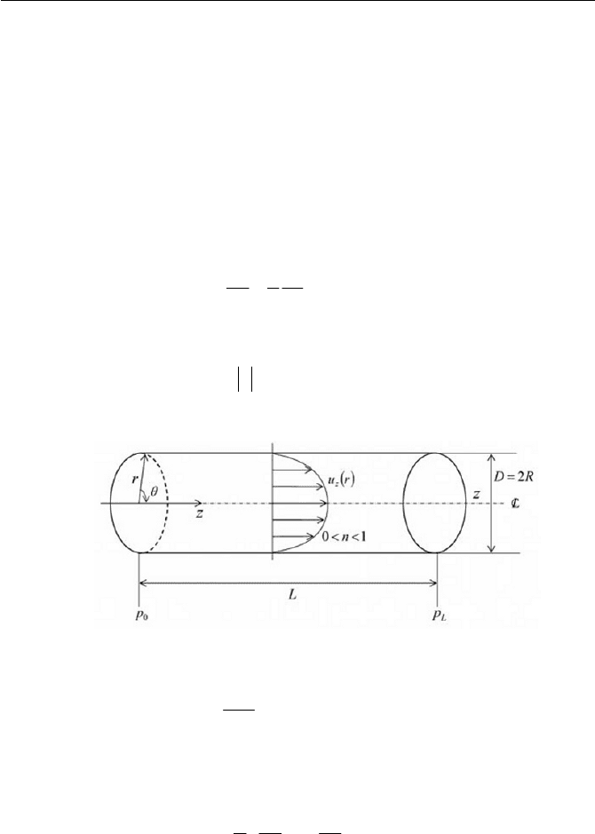
Exercise 7.1.2 Power Law Fluid in a Pipe
Consider the steady state laminar and isothermal flow in a horizontal pipe.
The fluid in the pipe is incompressible and can be treated by the power law
fluid. Find the fully developed flow velocity profile at an arbitrary cross
section of the pipe, and calculate the relevant flow properties, such as the
flow rate, the average velocity and the pressure drop along the pipe.
2
409
7 Non-Newtonian Fluid and Flow
Ans.
Assume that the flow is axisymmetric so that the velocity components
in the cylindrical coordinates
),,( zr
T
are
),,(
z
u00 u
(1)
where
z
u is the axial velocity component and is an only function of
r
as
depicted in Fig. 7.3. Ignoring the inertial and body force term, the
rz
r
rrz
p
W
w
w
w
w
1
0
(2)
The component of the shear stress
IJ
is given by the power law
JJW
1
n
rz
m
(3)
where
J
is the shear rate
rz
JJ
, and which is given as
Fig. 7.3 Pipe flow of power law fluid
r
u
z
w
w
J
(4)
Equation (2) can be integrated to obtain
rz
W
by the separation of vari-
ables so that we have
r
C
r
z
p
rz
1
2
1
¸
¹
·
¨
©
§
w
w
W
(5)
where
1
C is a constant. Since
rz
W
has a finite value at the center line, i.e.
0
r ,
1
C must be zero.
From Eqs. (3), (4) and (5), we can write an equation for
z
u
where
Cauchy's equation of motion in the unidirectional flow (
z directional) is
written to show
410
Exercise
r
z
p
r
u
r
u
m
n
z
¸
¹
·
¨
©
§
w
w
¸
¹
·
¨
©
§
w
w
w
w
2
1
1
᧹
ᨶ
(6)
Note that in the pipe flow we take the sign convention for a negative,
since the velocity gradient
ru
z
ww and the pressure gradient zp ww are
both negative. Equation (6) is now integrated for
z
u
by a separation of
variables as follows
n
z
r
z
p
mr
u
1
2
1
¿
¾
½
¯
®
¸
¹
·
¨
©
§
w
w
w
w
(7)
and
2
1
1
2
1
1
Cr
z
p
mn
n
u
n
n
n
z
¿
¾
½
¯
®
¸
¹
·
¨
©
§
w
w
(8)
where
2
C is a constant that is obtained by the boundary condition, i.e.
0᧹Ru
z
. Resultantly, the velocity profile
z
u
will be given where
»
»
»
¼
º
«
«
«
¬
ª
¸
¹
·
¨
©
§
¿
¾
½
¯
®
¸
¹
·
¨
©
§
w
w
n
n
z
R
r
R
z
p
mn
n
u
n
n
n
1
1
2
1
1
1
1
(9)
The speed at the axis is to be the maximum speed
max
U and is given by the
setting 0 r to yield
n
n
n
R
z
p
mn
n
U
max
1
1
2
1
1
»
¼
º
«
¬
ª
¸
¹
·
¨
©
§
w
w
(10)
As a result, the velocity profile
z
u will now be alternatively expressed
with
max
U as follows
»
»
»
¼
º
«
«
«
¬
ª
¸
¹
·
¨
©
§
n
n
maxz
r
Uu
1
R
1
(11)
The flow rate
Q is thus calculated by integrating
z
u across the radius to
give
411
7 Non-Newtonian Fluid and Flow
max
R
z
UR
n
n
r druQ
2
0
13
1
2
SS
³
(12)
The average velocity
u is also obtained from Eq. (12) where
max
2
13
1
U
n
n
R
Q
u
S
(13)
The pressure gradient
zp ww is constant along the
z
axis, which is given
by
L
p
L
pp
z
p
L
w
w
0
(14)
where
p is the pressure drop, leaving 0!p . Using Eq. (14), the
(Darcy) friction factor
O
, p is obtained by
>@
¸
¹
·
¨
©
§
¸
¹
·
¨
©
§
¸
¹
·
¨
©
§
¸
¹
·
¨
©
§
2
2
2
11328
2
1
u
d
L
Re
nn
u
d
L
p
n
U
UO
*
/
(15)
*
Re is the generalized Reynolds number defined in Eq. (7.1.27)
Note that the velocity distribution given in Eq. (11) shows flatter near
the axis due to shear thinning, i.e.
10 n . As 1on , when the Poiseuille
paraboloid tends to persist, and when 1 n the friction factor becomes
Re/64
O
.
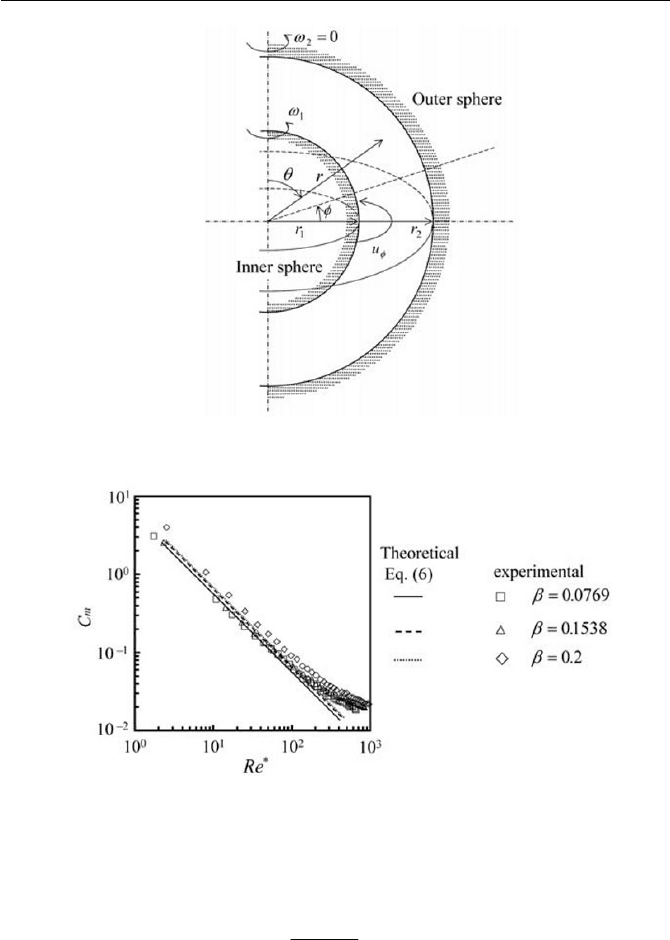
Exercise 7.1.3 Spherical Gap Flow with Power Law Fluid
Examine the flow of power law fluid contained in a gap between two con-
centric spheres, where the inner sphere rotates at a given constant angular
velocity
Z
, while the outer sphere is kept stationary. Assume that the gap
is sufficiently narrow so that the simple shear flow persists, referring to
section 6.3.1. Find the unidirectional velocity profile
ru
I
and the torque
to rotate the inner sphere against the frictional force. The geometric con-
figuration is shown in Fig. 7.4.
Let
I
u be the circumferential velocity (velocity component of
I
direc-
tion) and be the only function for
r
, i.e.
I
u,,00 u
and
ruu
II
, as in-
dicated in Fig. 7.4. By ignoring the inertial term and the body force term,
the pressure gradient in the circumferential direction (
I
direction) is null
'
'
'
'
'
412
Exercise
due to the symmetry, provided that only the Cauchy’s equation of motion
in the circumferential direction is written where
I
W
r
r
r
r
3
3
w
w
1
0
(1)
The shear stress
I
W
r
is given where the power law gives
JJW
I
1
n
r
m
(2)
J
is the shear rate
I
J
J
r
, which is written as
¸
¹
·
¨
©
§
w
w
r
u
r
r
I
J
(3)
Equation (1), together with Eqs. (2) and (3), is then solved with the bound-
ary conditions:
11
for rrru
Z
I
(4)
and
2
for0 rru
I
(5)
These give the solution for
I
u , as follows
»
»
¼
º
«
«
¬
ª
¸
¹
·
¨
©
§
»
»
¼
º
«
«
¬
ª
1
1
11
3
1
3
n
n
rr
r
u
/
/
/
E
E
Z
I
(6)
Note that in Eq. (6),
E
is the gap ratio defined as
1
12
r
rr
E
(7)
The net toque
r
T needed to rotate the inner sphere is governed by the shear
stress
I
W
r
acting on the inner sphere; this is calculated by integrating
I
W
r
over the inner sphere with
TTWS
S
I
drT
rr
2
0
3
1
sin2
³
(8)
Note that Eq. (8) is valid for an axisymmetric flow, i.e.
0 ww
I
, in gen-
eral without
II
W
contribution.
413
7 Non-Newtonian Fluid and Flow
Fig. 7.4 Flow of a power law fluid between concentric rotating spheres
Fig. 7.5 Torque characteristic in a spherical gap flow
It is often convenient to nondimensionalize the torque
r
T in such a way
that
2
1
5
1
ZU
r
T
C
r
m
(9)
where
U
is the liquid density and
m
C is called the torque coefficient. Sub-
stituting Eq. (6) for Eq. (3), as well as for Eq. (2), we can obtain the torque
coefficient
m
C through Eqs. (8) and (9), as follows
414