Wilkinson D.J. Stochastic Modelling for Systems Biology
Подождите немного. Документ загружается.

204
BAYESIAN INFERENCE AND MCMC
3.
Change
counter
j
to
j +
1,
and
return
to
step
2.
This clearly defines a homogeneous Markov chain, as each simulated value depends
only on the previous simulated value, and not on any other previous values or the
iteration counter
j.
However, we need to show that
1r(B)
is a stationary distribution
of
this chain. The transition kernel
of
the chain is
d
p(B,¢)
=II
7r(¢ij¢1,
...
,¢i-l,Bi+l,•··,Bd)·
i=l
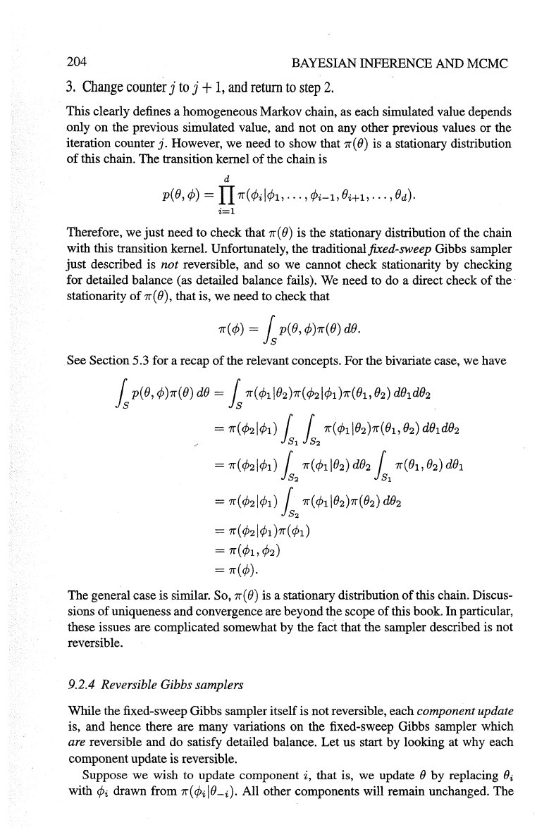
Therefore, we just need to check that
1r(
B)
is the stationary distribution
of
the chain
with this transition kernel. Unfortunately, the traditional
fixed-sweep Gibbs sampler
just described is
not
reversible, and so we cannot check stationarity by checking
for detailed balance (as detailed balance fails).
We
need to do a direct check
of
the·
stationarity
of
1r(
B),
that is, we need to check that
1r(¢)
=is
p(B,
¢)1r(B)
dB.
See Section 5.3 for a recap
of
the relevant concepts. For the bivariate case, we have
isp(B,¢)1r(B)dB
=is
7r(¢1JBz)7r(¢zJ¢1)7r(B
1
,Bz)dB
1
dB
2
=7r(¢zJ¢1)
{ {
7r(¢1JBz)1r(B1,Bz)dB1dBz
Js1
ls2
=
7r(¢zJ¢1)
{
1r(¢1JBz)dBz
{
1r(B1,Bz)dB1
Js2
Jsl
=
1r(¢zJ¢1)
{
1r(¢1JBz)1r(Bz)
dBz
ls2
=
1r(
¢zJ¢1
)1r(
¢1)
= 1r(¢1,¢2)
=
7r(¢).
The general case is similar. So,
1r(
B)
is a stationary distribution
of
this chain. Discus-
sions
of
uniqueness and convergence are beyond the scope
of
this book. In particular,
these issues are complicated somewhat by the fact that the sampler described is not
reversible.
9.2.4 Reversible Gibbs samplers
While the fixed-sweep Gibbs sampler itself is not reversible, each component update
is, and hence there are many variations on the fixed-sweep Gibbs sampler which
are reversible and do satisfy detailed balance. Let us start by looking at why each
component update is reversible.
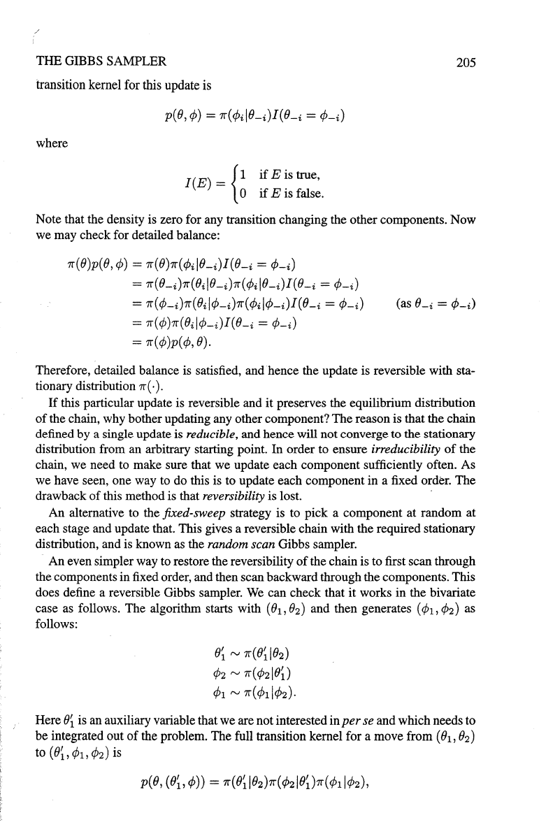
Suppose we wish to update component
i,
that is, we update B by replacing
Bi
with ¢i drawn from 7r(¢iJB-i)· All other components will remain unchanged. The
206
BAYESIAN INFERENCE AND MCMC
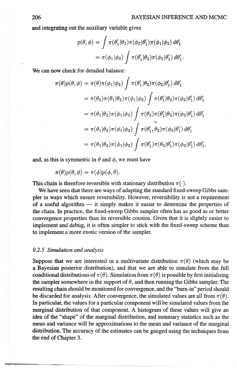
and
integrating
out
the auxiliary variable gives
p(B,¢) = j
7r(B~IB2)7r(¢2IBD1r(¢1l¢2)dB~
=
1r(¢1l1>2)
j
1r(B~IB2)7r(¢2IB~)
dB~.
We can now check for detailed balance:
7r(
B)p(
(}'
1>)
=
7r(
0)7r(
¢11¢2)
J
7r(
(}~
IB2
)7r(
¢2IBD
d(}~
=
7r(B2)7r(BIIB2)7r(¢II¢2)
j
1r(B~IB2)7r(¢2IBD
dB~
=
1r(
B1IB2)1r(
1>1l1>2)
j
1r(B2)1r(B~
1Bz)7r(
1>2IBD
dB~
=
1r(BIIB2)7r(¢1l¢2)
j
1r(B~,;2)1r(¢2IB~)
dB~
=
1r(BIIB2)1r(¢II1>2)
j
7r(B~)7r(02IBD7r(¢2IBDdB~,
and, as this
is
symmetric in B and ¢,
we
must have
1r(B)p(B,
1>)
= 1r(¢)p(¢,
B).
This chain is therefore reversible with stationary distribution
1r(
·).
We have seen that there are ways
of
adapting the standard fixed-sweep Gibbs sam-
pler in ways which ensure reversibility. However, reversibility is not a requirement
of
a useful algorithm - it simply makes
it
easier to determine the properties
of
the chain.
In
practice, the fixed-sweep Gibbs sampler often has as good
as
or
better
convergence properties than its reversible cousins. Given that
it
is slightly easier to
implement and debug, it is often simpler to stick with the fixed-sweep scheme than
to implement a more exotic version
of
the sampler.
9.2.5 Simulation and analysis
Suppose that
we
are interested in a multivariate distribution
1r(O)
(which may be
a Bayesian posterior distribution), and that
we
are able to simulate from the full
conditional distributions
of
1r(
B).
Simulation from
1r(
B)
is possible by first initialising
the sampler somewhere in the support
of
(},
and then running the Gibbs sampler. The
resulting chain should
be
monitored for convergence, and the "burn-in" period should
be
discarded for analysis. After convergence, the simulated values are all from
1r(
0).
In particular, the values for a particular component will
be
simulated values from the
marginal distribution
of
that component. A histogram
of
these values will give an
idea
of
the "shape"
of
the
marginal distribution, and summary statistics such as the
mean and variance will be approximations to the mean and variance
ofthe
marginal
distribution.
The
accuracy
of
the estimates can
be
gauged using the techniques from
tile end
of
Chapter 3.
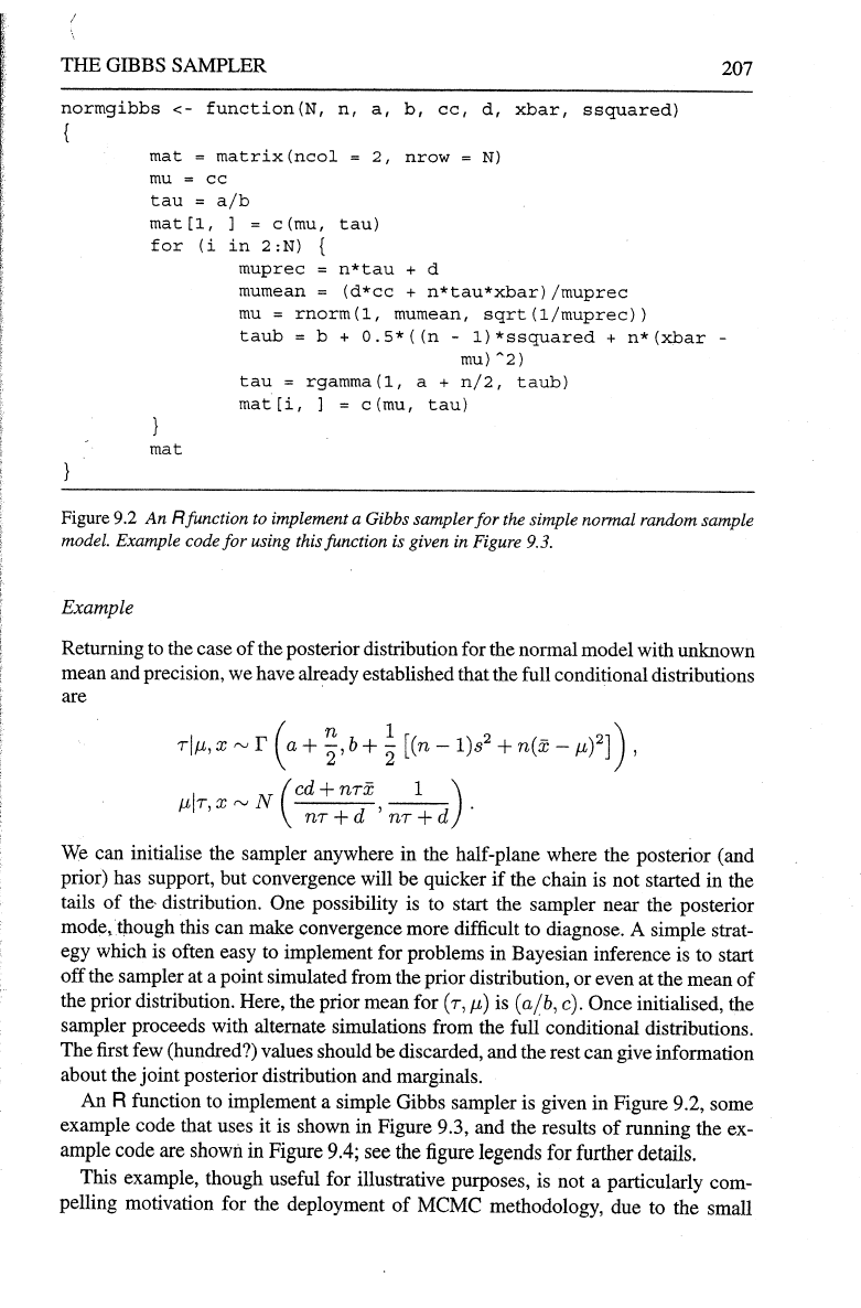
208
BAYESIAN INFERENCE AND MCMC
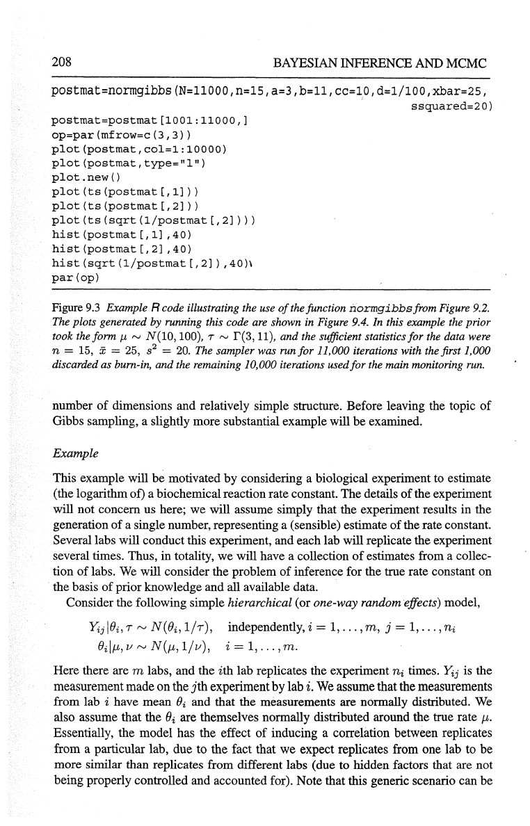
postmat=normgibbs(N=ll000,n=15,a=3,b=ll,cc=l0,d=l/lOO,xbar=25,
ssquared=20)
postmat=postmat[lOOl:llOOO,]
op=par(mfrow=c(3,3))
plot(postmat,col=l:lOOOO)
plot(postmat,type="l")
plot
.new
()
plot(ts(postmat[,l]))
plot(ts(postmat[,2]))
plot(ts(sqrt(l/postmat[,2])))
hist(postmat[,l]
,40)
hist(postmat[,2]
,40)
hist(sqrt(l/postmat[,2]),40)\
par(op)
Figure
9.3
Example R code illustrating the use
of
the function
normgibbsfrom
Figure 9.2.
The plots generated
by running this code
are
shown
in
Figure 9.4. In this example the prior
took the form
J.t
rv
N(10,
100), T
rv
r(3,
11), and the sufficient statistics
for
the data were
n
= 15, x = 25, s
2
=
20.
The sampler was run
for
11,000 iterations with the first 1,000
discarded as bum-in, and the remaining 10,000 iterations used for the main monitoring
run.
number
of
dimensions and relatively simple structure. Before leaving the topic of
Gibbs sampling, a slightly more substantial example will be examined.
Example
This example will be motivated by considering a biological experiment to estimate
(the logarithm of) a biochemical reaction rate constant. The details
of
the experiment
will not concern us here; we will assume simply that the experiment results in the
generation
of
a single number, representing a (sensible) estimate of the rate constant.
Several labs will conduct this experiment, and each lab will replicate the experiment
several times. Thus, in totality, we will have a collection
of
estimates from a collec-
tion
of
labs.
We
will consider the problem
of
inference for the true rate constant on
the basis
of
prior knowledge and all available data.
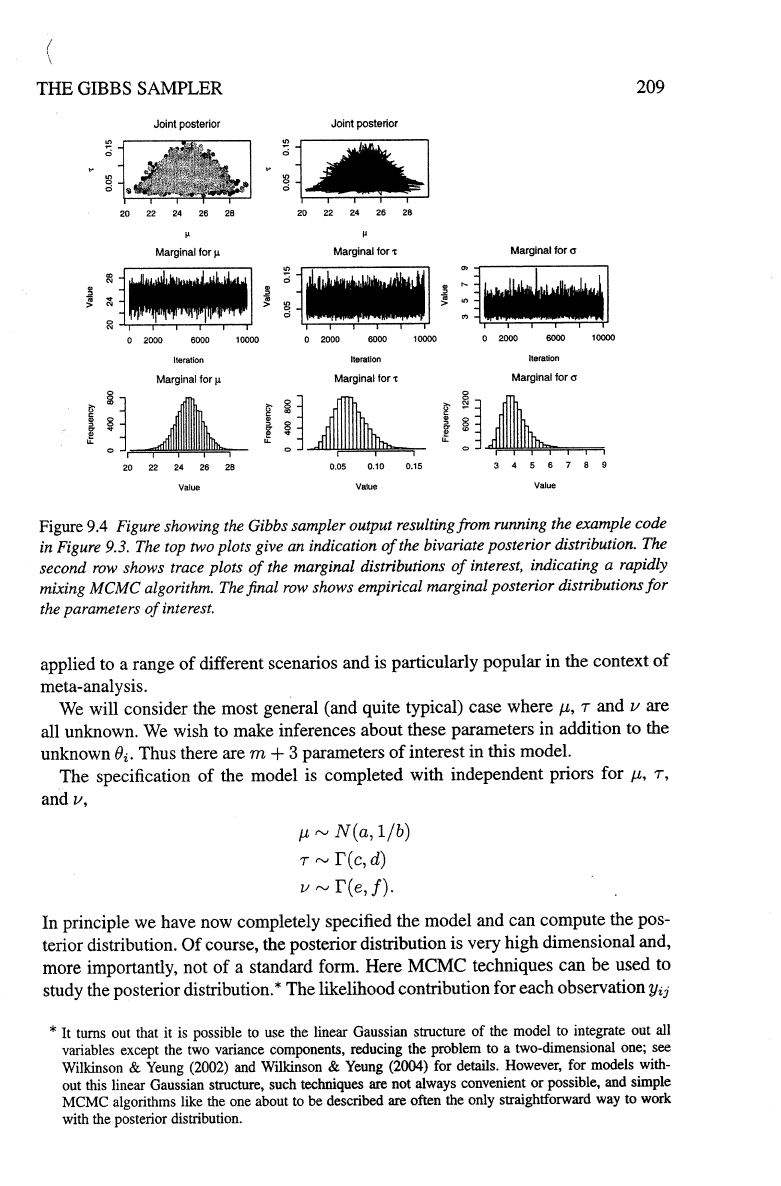
Consider the following simple
hierarchical (or one-way random effects) model,
Yij
IBi,
T"'
N(Bi,
1/r),
independently, i =
1,
...
,
m,
j =
1,
...
,
ni
Bdp,,
v"'
N(p,, 1/v), i =
1,
...
,
m.
Here there are m labs, and the ith lab replicates the experiment
ni
times.
Yij
is the
measurement made on the
jth
experiment by lab i.
We
assume that the measurements
from lab
i have mean
ei
and that the measurements are normally distributed.
We
also assume that the
ei
are themselves normally distributed around the true rate
p,.
Essentially, the model has the effect of inducing a correlation between replicates
from a particular lab, due to the fact that we expect replicates from one lab to be
more similar than replicates from different labs (due to hidden factors that are not
being properly controlled and accounted for). Note that this generic scenario can be

210
BAYESIAN
INFERENCE
AND
MCMC
is
L(O·
r
y·
·)·
-
{T
exp
{-:_(y·
·-
0·)
2
}
" ,
t]
- v
2:;:;:
2
tJ
t
and so the full likelihood is
m
ni
L(e,
T;
y)
=II
II
L(ei,
T;
YiJ)
where
i=l
j=l
(
T ) N
/2
{ T
~
2 2 }
= -
exp
-2
L_-
[(ni
-l)si
+
ni(Yi·-
8i) ]
2
7[
i=l
m
N=
l:ni,
i=l
1
n,
Yi·
= -
"'YiJ,
n·L-
'j=l
The prior takes the form
7r(J.-£,
T,
V,
())
=
7r(J.-£)7r(7)7r(v)7r(8lp,,
v)
where
1r(p,)
oc
exp
{
-~(p,-
a)
2
}
1r(T)
oc
Te-l
exp{
-dT}
1r(v)
oc
ve-l
exp{-
fv}
7r(BiiJ.-£,
v) =
~
exp
{
-~(ei-
J.-£?}
=>
1r(8lp,,
v)
oc
vm/
2
exp
{
-~
~(ei-
p,)
2
}
and therefore,
7r(J.-£,
T,
V,
())
OC
Ve+m/
2
-lTc-l
exp
{
-~
[ 2dT +
2fv
+
b(p,-
a)
2
+ V
~(()i
-
J.-£)
2
]}
· Now we have the likelihood and the prior, and we can write down the posterior
distribution,
7r(p,,
T,
v,
Bly)
()(
Tc+N/2-lve+m/2-1
exp
{ -
~
[ 2dT +
2fv
+
b(p,-
a)2
+
~
(v(ei-
p,)
2
+
T(ni-
l)sr
+
mi(Yi·-
ei)
2
)
J
}·
212
BAYESIAN INFERENCE AND MCMC
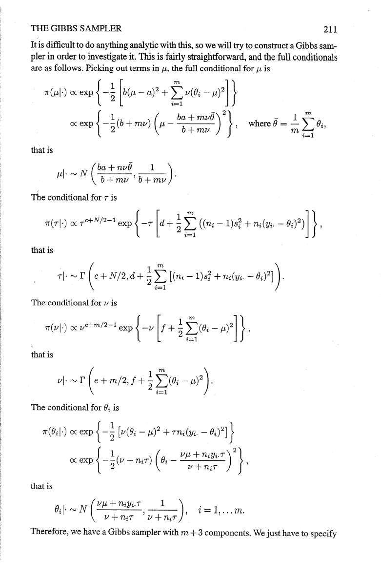
the
prior
parameters
a,
b,
c,
d,
e,
f
and
compute
the
data
summaries
m,
ni,
N,
Yi·,
si,
i = 1,
...
, m. Then we initialise the sampler by simulating from the prior, or by
starting off each component at its prior mean. The sampler is then run to convergence,
and samples from the stationary distribution are used to understand the marginals
of
the posterior distribution. This model is
of
sufficient complexity that assessing
convergence
of
the sampler
to
its stationary distribution is a non-trivial task. At the
very least, multiple large simulation runs are required, with different starting points,
and the first portion (say, a third)
of
any run should be discarded as "bum-in."
As
the complexity
of
the
model increases, problems with assessment
of
the convergence
of
the sampler also increase. There are many software tools available for MCMC
convergence diagnostics. R-CODA is an excellent package for
R which carries out a
range
of
output analysis and diagnostic tasks, but its use is beyond the scope
of
this
book.
It
is clear that in principle at least, it ought to be possible to automate the con-
struction
of
a Gibbs sampler from a specification containing the.model, the prior,
and the data. There are several freely available software packages that are able to
do this for relatively simple models. Examples include,
WinBUGS, OpenBugs, and
JAGS; see this book's website for links. Unfortunately, it turns out to be difficult to
use these software packages for the stochastic kinetic models that will be considered
in Chapter
10.
Of
course, the Gibbs sampler tacitly assumes that we have some reasonably ef-
ficient mechanism for simulating from the full conditional distributions, and yet
this is not always the case. Fortunately, the Gibbs sampler can be combined with
Metropolis-Hastings algorithms when the full conditionals are difficult
to
simulate
from.
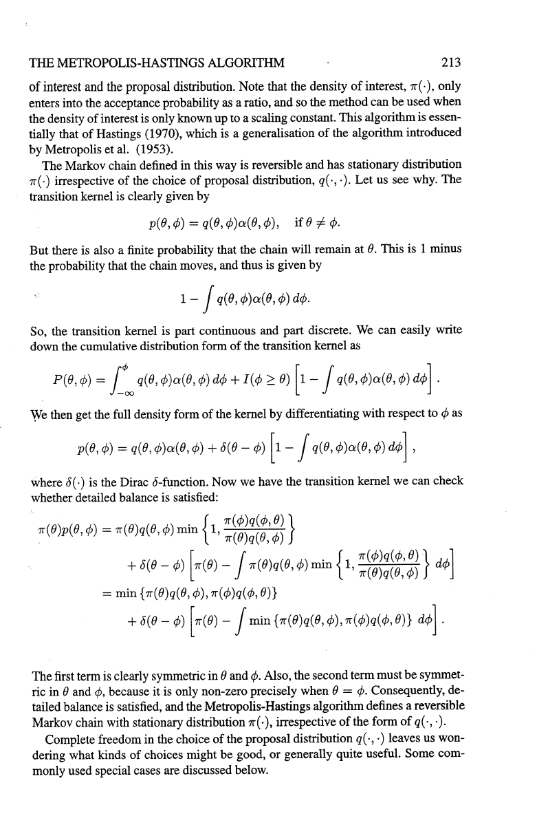
9.3 The Metropolis-Hastings algorithm
Suppose that
1r(
B)
is the density
of
interest. Suppose further that we have some (arbi-
trary) transition kernel q(B,
¢)
(known
as
the proposal distribution) which is easy to
simulate from, but does not (necessarily) have
1r(
B)
as
its stationary density. Consider
the following algorithm:
1.
Initialise the iteration counter to j = 1, and initialise the chain to B(o).
2.
Generate a proposed
value¢
using the kernel q(BU-
1
),
¢).
3.
Evaluate the acceptance probability
a(
BU:-
1
),
¢)
of
the proposed move, where
. {
7r(¢)q(¢,B)}
a(B,
¢)
=
mm
1,
1r(B)q(B,
¢)
.
4. Put
B(j)
=¢with
probability
a(BU-
1
),
¢),and
put
B(j)
= BU-
1
)
otherwise.
5. Change the counter from
j to j + 1 and return to step 2.
In other words, at each stage, a new value is generated from the proposal distribution.
This is either accepted, in which case the chain moves, or rejected, in which case the
chain stays where it is. Whether or not the move is accepted or rejected depends on
an
acceptance probability which itself depends on the relationship between the density
