Wilkinson D.J. Stochastic Modelling for Systems Biology
Подождите немного. Документ загружается.

174
CASE STUDIES
n
I
~t
~--....-
/-
./
Time
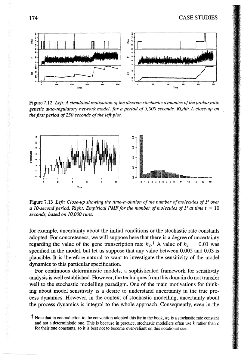
Figure
7.12
Left: A simulated realisation
of
the discrete stochastic dynamics
of
the prokaryotic
genetic auto-regulatory network model,
for
a period
of
5,000 seconds. Right: A close-up on
the first period
of
250 seconds
of
the left plot.
10
0
1 2 3 4 5 6 7 8 9
11
13 15
17
19
Time
Figure
7.
13
Left: Close-up showing the time-evolution
of
the number
of
molecules
of
P over
a
10-second period. Right: Empirical PMF for the number
of
molecules
of
Pat
timet
= 10
seconds, based on 10,000 runs.
for example, uncertainty about the initial conditions or the stochastic rate constants
adopted. For concreteness, we will suppose here that there is a degree
of
uncertainty
regarding the value
of
the gene transcription rate k
2
.t A value
of
k
2
= 0.01
was
specified in the model, but let us suppose that any value between 0.005 and 0.03 is
plausible.
It
is therefore natural to want to investigate the sensitivity of the model
dynamics to this particular specification.
For continuous deterministic models, a sophisticated framework for sensitivity
analysis is well established. However, the techniques from this domain
do
not transfer
well to the stochastic modelling paradigm.
One
of
the main motivations for think-
ing about model sensitivity is a desire to understand uncertainty in the true pro-
cess dynamics. However, in the context
of
stochastic modelling, uncertainty about
the process dynamics is integral to the whole approach. Consequently, even in the
t Note that in contradiction to the convention adopted this far in the book,
k2
is a stochastic rate constant
and not a deterministic one. This is because in practice, stochastic modellers often use
k rather than c
for their rate constants, so it is best not to become over-reliant on this notational cue.
AN
AUTO-REGULATORY
GENETIC
NETWORK
175
case
of
complete certainty regarding the model structure, rate laws, rate constants,
and initial conditions, the time-evolution
of
the process is uncertain (or random, or
stochastic, depending on choice
of
terminology). A natural way to incorporate un-
certainty regarding model parameters is to adopt a subjective Bayesian interpretation
of
probability. In the Bayesian paradigm, uncertainty regarding model parameters is
not fundamentally different to uncertainty regarding the time evolution
of
the process
due
to
the stochastic kinetic dynamics. We have already constructed mechanisms for
handling uncertainty in the process dynamics by trying to understand the probability
distribution
of
the outcomes, rather than by simply looking at a particular realisa-
tion
of
the process. There is no reason why these probability distributions should
not include uncertainty regarding the model parameters in addition to the uncertainty
induced by the stochastic kinetics. This is best illustrated by example.
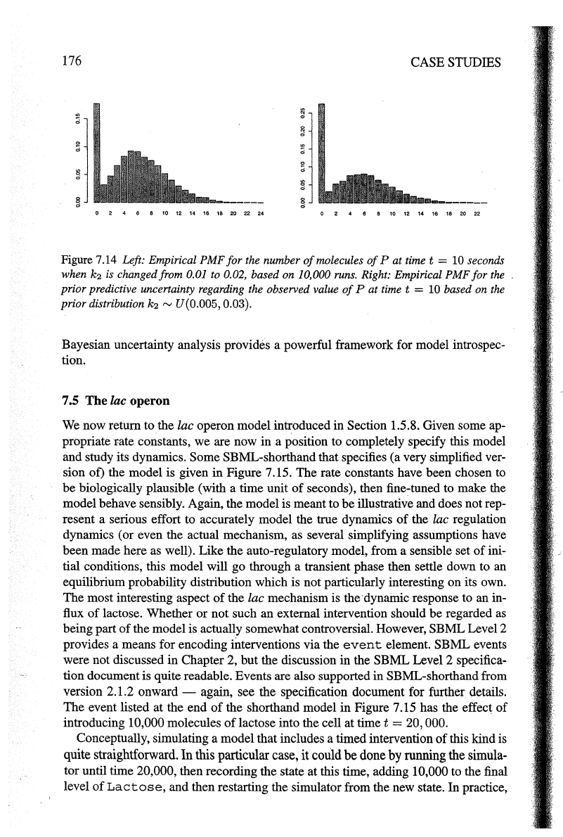
Figure 7.13 (right) shows our uncertainty about the level
of
Pat
timet=
10 based
on a
value
of
k
2
= 0.01. Similar plots can be produced based on other plausible val-
ues; Figure 7.14 (left) shows the plot corresponding to k
2
= 0.02, for example. In
order
to
obtain a summary
of
our uncertainty regarding the level
of
P,
we need to
average over our uncertainty for
k
2
in
an
appropriate way. In order to do this prop-
erly, we need
to
specify a probability distribution which reflects our uncertainty in
k
2
•
It
was previously stated that all values between 0.005 and 0.03 are plausible.
We will now make the much stronger assumption that all values in this range are
equally plausible, which leads directly
to
the probability distribution U(0.005, 0.3).
Within the Bayesian framework, this is known
as
a prior probability distribution for
a parameter.
t Having specified the prior probability distribution (in practice, there is
likely to be uncertainty regarding several parameters, but it is completely straightfor-
ward
to
assign independent prior probability distributions to each uncertain value), it
is then straightforward
to
incorporate this into the subsequent analysis. Rather than
running many simulations with the same parameters, each run begins by first picking
uncertain parameters from their prior probability distributions. This has the effect
of
correctly embedding the parameter uncertainty into the model; all subsequent anal-
ysis then proceeds as normal. For example,
if
interest is in the level
of
P at time
t = 10, the values can be recorded at the end
of
each run to build up a picture
of
the
marginal uncertainty for the level
of
P. Such a distribution is depicted in Figure 7.14
(right). Unsurprisingly, it looks a bit like a compromise between Figure 7.13 (right)
and Figure 7.14 (left).
In practice one is not simply interested in the uncertainty
of
the level
of
one par-
ticular biochemical species at one particular time, but it
is
clear that exactly the same
approach can be applied to any numerical summary
of
the simulation output (for ex-
ample, cell-cycle time, time
to
cell death, population doubling time, time for RNA
expression levels to increase five-fold, etc.). When applied to derived simulation out-
puts
of
genuine biological interest (possibly directly experimentally measurable),
:j:
It
is known
as
a prior distribution because it is possible
to
use tbe model and experimental data to
update tbis prior distribution into a
posterior
distribution, which describes the uncertainty regarding
tbe parameter having utilised the information in the data. This is
Bayesian
statistics,
and it will be
discussed futtber in tbe final chapters
of
tbis book.
176
CASE STUDIES
0 2 4 6 8 10 u 14 16 18
~ ~ ~
o 2 4 a a 10
tt
14 16 18
~
~
Figure 7.14 Left: Empirical PMF
for
the
number
of
molecules
of
Pat
timet=
10 seconds
when
k2
is changed from 0.01 to 0.02,
based
on
10,000 runs. Right: Empirical
PMF
for
the
prior
predictive uncertainty regarding the observed value
of
P
at
time t = 10 based
on
the
prior
distribution k2
rv
U(0.005, 0.03).
Bayesian uncertainty analysis provides a powerful framework for model introspec-
tion.
7.5 The lac operon
We now return
to
the lac operon model introduced in Section 1.5.8. Given some ap-
propriate
:rate
constants, we are now
in
a position to completely specify this model
and study its dynamics.
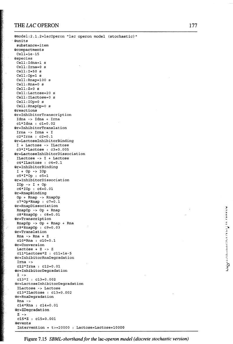
Some SBML-shorthand that specifies (a very simplified ver-
sion of) the model is given in Figure 7.15. The rate constants have been chosen
to
be
biologically plausible (with a time unit
of
seconds), then
fine~tuned
to make the
model behave sensibly. Again, the model is meant
to
be
illustrative and does not rep-
resent a serious effort to accurately model the true dynamics
of
the lac regulation
dynamics (or even the actual mechanism, as several simplifying assumptions have
been made here as well). Like the auto-regulatory model, from a sensible set
of
ini-
tial conditions, this model will
go
through a transient phase then settle down to an
equilibrium probability distribution which is
not
particularly interesting on its own.
The
most interesting aspect
of
the lac mechanism is the· dynamic response to an in-
flux
of
lactose. Whether
or
not such an external intervention should
be
regarded as
being part
of
the model is actually somewhat controversial. However, SBML
Level2
provides a means for encoding interventions via the
event
element. SBML events
were not discussed
in
Chapter 2, but the discussion in the SBML Level 2 specifica-
tion document is quite readable. Events are also supported in SBML-shorthand from
version 2.1.2 onward - again, see the specification document for further details.
The
event listed at the end
of
the shorthand model
in
Figure 7.15 has the effect
of
introducing 10,000 molecules
oflactose
into the cell at
timet=
20,000.
Conceptually, simulating a model that includes a timed intervention
of
this kind is
quite
straightforward.
In
this
particular
case,
it
coUld
be
done
by
running
the
simula-
tor until time 20,000, then recording the state
at
this time,
addi.Dg
10,000 to the final
level
of
Lactose,
and then restarting the simulator from the new state.
In
practice,
THE
LAC
OPERON
®model:2.1.2=lac0peron
"lac
operon
model
(stochastic)"
·®units
substance=item
®compartments
Cell=1e-15
®species
Cell:Idna=l
s
Cell.:
Irna=O
s
Cell:I•50
s
Cell:Op=1
s
Cell:Rnap=100
s
Cell:Rna=O
s
Cell
:Z=O
s
Cell:Lactose=20
s
Cell:ILactose=O
s
Cell
:
IOp=O
s
Cell:RnapOp=O s
®reactions
®r=IrihibitorTranscription
Idna
->
Idna
+
Irna
cl*Idna
:
cl=0.02
®r=InhibitorTranslation
Irna
->
Irna
+ I
c2*Irna
:
c2=0.1
®r=LactoseinhibitorBinding
I +
Lactose
->
!Lactose
c3*I*Lactose
:
c3=0.005
®r=LactoseinhibitorDissociation
!Lactose
->
I +
Lactose
c4*ILactose
:
c4=0.1
®r=InhibitorBinding
I +
0p
->
IOp
c5*I*Op : c5=1
®r=InhibitorDissociation
IOp
->
I +
Op
c6*IOp :
c6=0.01
®r=RnapBinding
Op
+ Rnap
->
RnapOp
c7*0p*Rnap :
c7=0.1
®r=RnapDissociation
Rna
pOp
->
Op
+ Rnap
cS*RnapOp :
c8=0.01
®r=Transcription
RnapOp
->
Op
+ Rnap + Rna
c9*Rnap0p :
c9=0.03
®r=Translation
Rna
->
Rna + z
clO*Rna :
cl0=0.1
®r=Conversion
Lactose
+ z
->
z
cll*Lactose*Z
:
cll=le-5
®r=InhibitorRnaDegradation
Irna
->
cl2*Irna
:
c12=0.01
®r=InhibitorDegradation
I
->
Cl3*I
:
cl3=0.002
®r=LactoseinhibitorDegradation
ILactose
->
Lactose
cl3*ILactose
:
cl3=0.002
®r=RnaDegradation
Rna
->
cl4*Rna
:
cl4=0.01
®r=ZDegradation
z
->
cl5*Z
:
cl5=0.001
®events
Intervention
=
t>=20000
: Lactose=Lactose+lOOOO
Figure
7.15
SBML-shorthandfor the
lac-operon
model (discrete stochastic version)
177
:r
:>
"
..
:r.
::=-
,)
..
,,
,l'
...
·•
.
..
:l
·~
:~
178
CASE STUDIES
.,
~
"'
~
~
-'
0
~
"'
~
c:
a:
"'
~
N
~
~
10000
20000 30000 40000
50000
Time
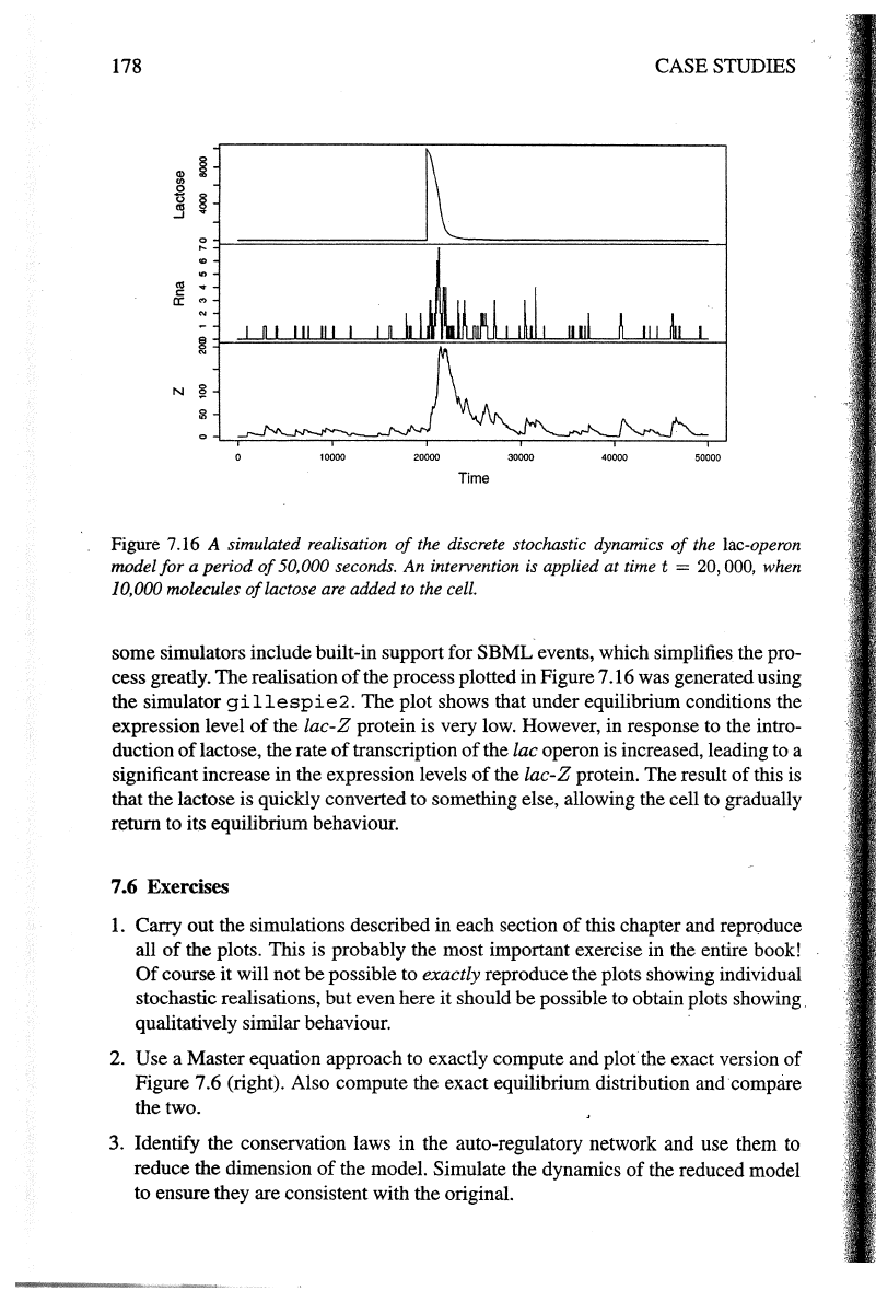
Figure 7.16 A simulated realisation
of
the discrete stochastic dynamics
of
the lac-operon
model for a period
of
50,000 seconds.
An
intervention is applied at time t = 20, 000, when
10,000 molecules
of
lactose are added to the cell.
some simulators include built-in support for SBML events, which simplifies the pro-
cess greatly. The realisation
of
the process plotted in Figure 7.16 was generated using
the simulator
gillespie2.
The plot shows that under equilibrium conditions the
expression level
of
the lac-Z protein is very low. However, in response to the intro-
duction
of
lactose, the rate
of
transcription
of
the lac operon is increased, leading to a
significant increase in the expression levels
of
the
lac-Z
protein. The result
of
this
is
that the lactose is quickly converted to something else, allowing the cell to gradually
return to its equilibrium behaviour.
7.6 Exercises
1.
Carry out the simulations described in each section
of
this chapter and reproduce
all
of
the plots. This is probably the most important exercise in the entire book!
Of
course
it
will not be possible to exactly reproduce the plots showing individual
stochastic realisations, but even here it should be possible to obtain plots showing.
qualitatively similar behaviour.
2.
Use a Master equation approach to exactly compute and
plotthe
exact version
of
Figure 7.6 (right). Also compute the exact equilibrium distribution and compare
the two.
3. Identify the conservation laws in the auto-regulatory network and use them
to
reduce the dimension
of
the model. Simulate the dynamics
of
the reduced model
to ensure they are consistent with the original.
FlJRii.HER READING
179
4. Deduce the continuous deterministic version
of
the auto-regulatory model ( assum-
ing a container volume
of
10-
15
L) and simulate it. Compare
it
to the stochastic
version. How well does it describe the mean behaviour
of
the stochastic version?
5.
In the dimerisation kinetics ·model, the dissociation rate constant c
2
took the value
0.2. Suppose now that there is uncertainty regarding this value which can
be
well
described by a
U(O.l, 0.4) probability distribution. Produce a new version
of
Fig-
ure 7.6 (right) which incorporates this uncertainty.
7.7
Further reading
This chapter provides only the briefest
of
introductions to stochastic modelling
of
genetic and biochemical networks, but it should provide sufficient background in or-
der to render the literature in this area more accessible.
To
build large and complex
stochastic models
of
interesting biological processes, it is necessary to read around
the deterministic modelling literature in addition to the
stochastic literature, as the
deterministic literature is much more extensive, and can still provide useful informa-
tion for building stochastic models.
Good
starting points include Bower & Bolouri
(2000), Kitano (2001) and Klipp et al. (2005); also see the references therein. The
existing literature on stochastic modelling is
of
course particularly valuable, and I
have found the following articles especially interesting: McAdams & Arkin (1997),
Arkin
et
al. (1998), McAdams & Arkin (1999), Goss & Peccoud (1998), Pinney et al.
(2003), Hardy & Robillard (2004), Salis & Kaznessis (2005b). Readers with an in-
terest in stochastic modelling
of
aging mechanisms might also like to read Proctor
et al.
(2005). In addition to the modelling literature; it is invariably necessary to
trawl the wet-biology literature and online databases
f()r
information on mechanisms
and kinetics - mastering this process is left as an additional exercise for the reader,
though some guidance is provided in Klipp et al.
(2005).

CHAPTERS
Beyond the Gillespie algorithm
8.1 Introduction
In Chapter 6 an algorithm for simulating the time-course behaviour
of
a stochastic
kinetic model was introduced. This discrete-event simulation algorithm, usually re-
ferred· to as the Gillespie algorithm, has the nice properties that it simulates every re-
action event and is exact in the sense that it generates exact independent realisations
of
the underlying stochastic kinetic model.
It
is also reasonably efficient in terms
of
computation time among all such algorithms with those properties. However,
it
sho~d
be
emphasised that the Gillespie algorithm is
just
one approach out
of
many
that could
be
taken to simulating stochastic biochemical dynamics. In this chapter
we will look at some other possible approaches, motivated by problems in apply-
ing the Gillespie algorithm to large models containing species with large numbers
of
molecules and fast reactions.
In
Section 8.2, refinements
of
the Gillespie algorithm
will be considered that still generate exact realisations
of
the stochastic kinetic pro-
cess. In Section 8.3, methods based on approximating the process by another that
is faster to simulate will
be
examined. Then in Section 8.4, hybrid algorithms that
combine both exact and approximate updating strategies will
be
considered.
8.2 Exact simulation methods
Let us begin by reconsidering discrete event simulation
of
a continuous time Markov
process with a finite number
of
states, as described
in
Section 5.4 (p. 121). We saw
how to do this using the direct method in Section
5.4.2. There is an alternative algo-
rithm to this, known as the first event method, which also generates an exact realisa-
tion
of
the Markov process.
It
can
be
stated as follows:
1.
Initialise the process at t = 0
With
initial state i.
2.
Call the current state i. For each potential other state k (k
=/=
i), compute a putative
time to transition to that state
tk
""Exp(qik).
3.
Let
j
be
the index
of
the smallest
of
the
tk.
4.
Putt
: = t +
tj.
5.
Let the new state
be
j.
6. Output the time t and state
j.
7.
1ft<
Tmax•
return to step 2.
It
is perhaps not immediately obvious that this algorithm is exactly equivalent to the
direct method. In order to see that
it
is, we need to recall some relevant properties
181
:">
182 BEYOND
THE
GILLESPIE ALGORITIIM
of
the exponential distribution; presented in Section 3.9 (p. 77).
By
Proposition 3.18,
the
minimum
of
the putative times has the correct distribution for the time to the first
event, and
by
Proposition 3.19, the index associated with that minimum time clearly
has the correct probability mass function
(PMF).
Although the first event method is
just
as correct as the direct method, the direct
method is generally to
be
preferred, as it is more efficient. In particular, the direct
method requires
just
two random numbers to be simulated
per
event, whereas the
first event method requires
r (where r is the number
of
states). The first event method
is interesting, however, as it gives us another way
of
thinking about the simulation
of
the process, and forms the basis
of
a very efficient exact simulation algorithm for
stochastic kinetic models.
8.2.1 First reaction method
Before looking
at
the Gibson-Brock algorithm in detail, it is worth thinking briefly
about how the first event method for finite state Markov processes translates to
stochastic kinetic models with a potentially infinite state space. We have already
seen how the direct method translates into the Gillespie algorithm (Section 6.4). The
first event method translates into a variant
of
the Gillespie algorithm known as the
first reaction method (Gillespie 1976), which can be stated as follows:
1.
Initialise the starting point
of
the simulation with t : = 0, rate constants c =
(Ct.
...
,
Cv)
and initial state x = (
Xt.
...
,
x,..).
2. Calculate the reaction hazards hi(x, ci), i = 1, 2,
...
,
v.
3. Simulate a putative time to the next type i reaction,
ti
"'
Exp(hi(x,
q)),
i =
1,2,
...
,v.
4. Let j
be
the index
of
the smallest
ti.
5.
Putt
: = t +
tj.
6. Update the state x according to the reaction with index
j.
That is, set x : = x +
s(j).
7; Output t and x.
8.
If
t < T
max
return to step 2.
As stated, this algorithm is clearly less efficient than Gillespie's direct method, but
with a few clever tricks it can
be
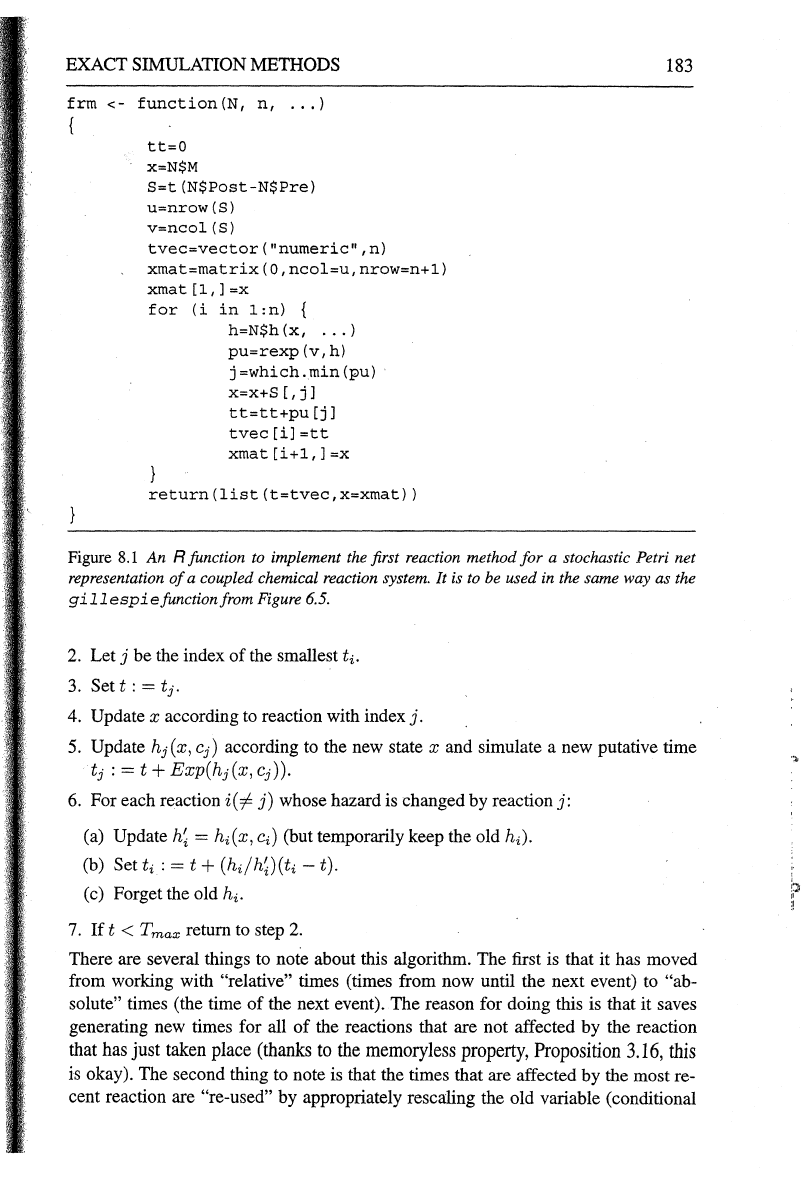
turned into a very efficient algorithm. An R function
to implement the first reaction method for a
SPN is given in Figure 8.1.
8.2.2 The Gibson-Bruck algorithm
The so-called next reaction method (also known as the Gibson-Brock algorithm)
i~
a
modification
of
the first reaction method which makes it much more efficient. A first
attempt
at
presenting the basics
of
the Gibson-Brock algorithm follows:
1. Initialise
t : = 0, c and x, and additionally calculate all
of
the initial reaction haz-
ards hi(x,
q),
i = 1,
...
, v. Use these hazards to simulate putative first reaction
times
ti
rv
Exp(hi(x,
Ci)).
EXACT SIMULATION METHODS
frm
<-
function(N,
n,
...
)
tt=O
x=N$M
S=t(N$Post-N$Pre)
u=nrow(S)
v=ncol(S)
tvec=vector
("numeric",
n)
xmat=matrix(O,ncol=u,nrow=n+l)
xmat[l,]=x
for
(i
in
l:n)
{
h=N$h(x,
...
)
pu=rexp(v,h)
j=which.min(pu)
X=X+S
(,
j]
tt=tt+pu
[j]
tvec[i]=tt
xmat[i+l,]=x
return(list(t=tvec,x=xmat))
183
Figure
8.1
An R function to implement the first reaction method for a stochastic Petri net
representation
of
a coupled chemical reaction system. It is
to
be
used in the same way as the
gillespiefunctionfrom
Figure
6.5.
2.
Let j be the index of the smallest ti.
3.
Sett:
= t
1
.
4.
Update x according
to
reaction with index
j.
5.
Update hJ(x,
cJ)
according to the new state x and simulate a new putative time
tJ
: = t +
Exp(h
1
(x,
c
1
)).
6.
For each reaction i(
"1-
j)
whose hazard is changed by reaction j:
(a) Update
h~
=
hi(x,
ci) (but temporarily keep the old hi).
(b) Set ti : = t +
(h;jh~)(ti-
t).
(c) Forget the old hi.
7.
If t < T
max
return to step
2.
There are several things to note about this algorithm. The first is that it has moved
from working with
"relative" times (times from now until the next event)
to
"ab-
solute"
times (the time
of
the next event). The reason for doing this is that it saves
generating new times for all
of
the reactions that are not affected by the reaction
that has just taken place (thanks
to
the memoryless property, Proposition
3.16,
this
is okay). The second thing to note is that the times that are affected by the most re-
cent reaction are
"re-used" by appropriately rescaling the old variable (conditional
.,
