White R.E. Computational Mathematics: Models, Methods, and Analysis with MATLAB and MPI
Подождите немного. Документ загружается.


1.3. DIFFUSION IN A WIRE WITH LITTLE INSULATION 17
Since
D
n
converges to the zero matrix, the column vectors x
n+1
x must con-
verge to the zero column vector.
1.2.7 Exercises
1.
2. In heat.m let
pd{n = 120 so that gw = 150@120 = 1=25. Experiment
with the space step sizes
g{ = =2> =1> =05 and q = 5> 10> 20, respectively.
3. In heat.m let
q = 10 so that g{ = =1. Experiment with time step sizes
gw = 5> 2=5> 1=25 and pd{n = 30> 60 and 120, respectively.
4. In heat.m experiment with di
erent values of the thermal conductivity
frqg = =002> =001 and .0005. Be sure to adjust the time s tep so that the stability
condition holds.
5. Consider the variation on the thin wire where heat is lost through the sur-
face of the wire. Modify heat.m and experiment with the
F and u parameters.
Explain your computed results.
6. Consider the variation on the thin wire where heat is generated by
i =
1 +
vlq(10w)= Modify heat.m and experiment with the parameters.
7. Consider the 3×3
D matrix for (1.2.1). Compute D
n
for n = 10> 100> 1000
for dierent values of alpha so that the stability condition either does or does
not hold.
8. Suppose
q = 5 so that there are 4 unknowns. Find the 4 × 4 matrix
version of the finite di
erence model (1.2.1). Repeat the previous problem for
the corresponding 4 × 4 matrix.
9. Justify the second and third lines in the displayed equations in the proof
of the Steady State Theorem.
10. Consider a variation of the Steady State Theorem where the column
vector
e depends on time, that is, e is replaced by e
n
. Formulate and prove a
generalization of this theorem.
1.3 Diusion in a Wire with Little Insulation
1.3.1 Intro duction
In this section we consider heat diusion in a thin electrical wire, which is not
thermally insulated on its lateral surface. The model of the temperature will
still have the form x
n+1
= Dx
n
+ e, but the matrix D and column vector e will
be dierent than in the insulated lateral surface model in the previous section.
1.3.2 Applied Area
In this section we present a third model of heat transfer. In our first model
we considered heat transfer via a discrete version of Newton’s law of cooling.
That is, we assumed the mass had uniform temperature with respect to space.
In the previous section we allowed the temperature to be a function of both
© 2004 by Chapman & Hall/CRC
Using the MATLAB code heat.m duplicate Figures 1.2.3-1.2.5.
18 CHAPTER 1. DISCRETE TIME-SPACE MODELS
discrete time and discrete space. Heat di
used via the Fourier heat law either
to the left or right direction in the wire. The wire was assumed to be perfectly
insulated in the lateral surface so that no heat was lost or gained through the
lateral sides of the wire. In this section we will allow heat to be lost through
the lateral surface via a Newton-like law of cooling.
1.3.3 Model
Discretize both space and time and let the temperature x(lk> nw) be approx-
imated by
x
n
l
where w = W @pd{n, k = O@q and O is the length of the wire.
The model will have the general form
change in heat in (
kD) (heat from the source)
+(di
usion through the left end)
+(di
usion through the right end)
+(heat loss through the lateral surface)
=
whose length is k and cross section is D = u
2
= So the lateral surface area is
k2u.
The heat loss through the lateral surface will be assumed to be directly
proportional to the product of change in time, the lateral surface area and to
the di
erence in the surrounding temperature and the temperature in the wire.
Let f
vxu
be the proportionality constant that measures insulation. If x
vxu
is
the surrounding temperature of the wire, then the heat loss through the small
lateral area is
f
vxu
w 2uk(x
vxu
x
n
l
)= (1.3.1)
Heat loss or gain from a source such as electrical current and from left and right
diusion will remain the same as in the previous section. By combining these
we have the following approximation of the change in the heat content for the
small volume Dk:
fx
n+1
l
Dk fx
n
l
Dk = Dk w i
+D w N(x
n
l+1
x
n
l
)@k D w N(x
n
l
x
n
l1
)@k
+f
vxu
w 2uk(x
vxu
x
n
l
) (1.3.2)
Now, divide by
fDk, define = (N@f)(w@k
2
) and explicitly solve for x
n+1
l
.
Explicit Finite Di
erence Model for Heat Diusion in a Wire.
x
n+1
l
= (w@f)(i + f
vxu
(2@u)x
vxu
) + (x
n
l+1
+ x
n
l1
)
+(1
2 (w@f)f
vxu
(2@u))x
n
l
(1.3.3)
for
l = 1> ===> q 1 and n = 0> ===> pd{n 1>
x
0
l
= 0 for l = 1> ===> q 1 (1.3.4)
x
n
0
= x
n
q
= 0 for n = 1> ===> pd{n= (1.3.5)
© 2004 by Chapman & Hall/CRC
This is depicted in the Figure 1.2.1 where the volume is ahorizontal cylinder
1.3. DIFFUSION IN A WIRE WITH LITTLE INSULATION 19
Equation (1.3.4) is the initial temperature set equal to zero, and (1.3.5) is the
temperature at the left and right ends set equal to zero. Equation (1.3.3) may
be put into the matrix version of the first order finite di
erence method. For
example, if the wire is divided into four equal parts, then n = 4 and (1.3.3) may
be written as three scalar equations for the unknowns x
n+1
1
> x
n+1
2
and x
n+1
3
:
x
n+1
1
= (w@f)(i + f
vxu
(2@u)x
vxu
) + (x
n
2
+ 0) +
(1
2 (w@f)f
vxu
(2@u))x
n
1
x
n+1
2
= (w@f)(i + f
vxu
(2@u)x
vxu
) + (x
n
3
+ x
n
1
) +
(1
2 (w@f)f
vxu
(2@u))x
n
2
x
n+1
3
= (w@f)(i + f
vxu
(2@u)x
vxu
) + (0 + x
n
2
) +
(1
2 (w@f)f
vxu
(2@u))x
n
3
=
These three scalar equations can be written as one 3D vector equation
x
n+1
= Dx
n
+ e where (1.3.6)
x
n
=
5
7
x
n
1
x
n
2
x
n
3
6
8
> e
= (w@f )I
5
7
1
1
1
6
8
>
D
=
5
7
1 2 g 0
1 2 g
0 1 2 g
6
8
and
I = i + f
vxu
(2@u)x
vxu
and g = (w@f)f
vxu
(2@u)=
An important restriction on the time step w is required to make sure the
algorithm is stable. For example, consider the case
q = 2 where equation (1.3.6)
is a scalar equation and we have the simplest first order finite dierence model.
Here
d = 1 2 g and we must require d ? 1. If d = 1 2 g A 0 and
> g A 0, then this condition will hold. If q is larger than 2, this simple condition
will imply that the matrix products
D
n
will converge to the zero matrix, and
this analysis will be presented later in Chapter 2.5.
Stability Condition for (1.3.3).
1 2(N@f)(w@k
2
) (w@f)f
vxu
(2@u) A 0=
Example. Let O = f = = 1=0> u = =05> q = 4 so that k = 1@4> N =
=001> f
vxu
= =0005> x
vxu
= 10= Then = (N@f)(w@k
2
) = (=001)w16 and g =
(w@f)f
vxu
(2@u) = w(=0005)(2@=05) so that 1 2(N@f)(w@k
2
) (w@f)f
vxu
(2@u) = 1 =032w w(=020) = 1 =052w A 0= Note if q increases to 20, then
the constraint on the time step will significantly ch ange.
1.3.4 Method
The numbers x
n+1
l
generated by equations (1.3.3)-(1.3.5) are hopefully good
approximations for the temperature at
{ = l{ and w = (n + 1)w= The tem-
perature is often denoted by the function
x({> w)= Again the x
n+1
l
will be stored
© 2004 by Chapman & Hall/CRC
20 CHAPTER 1. DISCRETE TIME-SPACE MODELS
in a two dimensional array, which is also denoted by
x but with integer indices
so that
x
n+1
l
= x(l> n+1) x(l{> (n+1)w) = temperature function. In order
to compute all x
n+1
l
, we must use a nested loop where the i-loop (space) is the
inner loop and the k-loop (time) is the outer loop. This is illustrated in the
x(l> n + 1) on the three previously computed
x(l 1> n) , x(l> n) and x(l + 1> n).
1.3.5 Implementation
A slightly modified version of heat.m is used to illustrated the e ect of changing
the insulation coe
!cient, f
vxu
. The implementation of the above model for
temperature that depends on both space and time will have nested loops where
the outer loop is for discrete time and the inner loop is for discrete space. In
the M
ATLA B code heat1d.m these nested loops are given in lines 33-37. Lines
1-29 contain the input data with additional data in lines 17-20. Here the radius
of the wire is u = =05, which is small relative to the length of the wire O = 1=0.
The surrounding temperature is x
vxu
= 10= so that heat is lost through the
lateral surface when
f
vxu
A 0. Lines 38-41 contain the output data in the form
of a surface plot for the temperature.
MATLAB Code heat1d.m
1. % This code models heat diusion in a thin wire.
2. % It executes the explicit finite dierence method.
3. clear;
4. L = 1.0; % length of the wire
5. T = 400.; % final time
6. maxk = 100; % number of time steps
7. dt = T/maxk;
8. n = 10.; % number of space steps
9. dx = L/n;
10. b = dt/(dx*dx);
11. cond = .001; % thermal conductivity
12. spheat = 1.0; % specific heat
13. rho = 1.; % density
14. a = cond/(spheat*rho);
15. alpha = a*b;
16. f = 1.; % internal heat source
17. dtc = dt/(spheat*rho);
18. csur = .0005; % insulation coe!cient
19. usur = -10; % surrounding temperature
20. r = .05; % radius of the wire
21. for i = 1:n+1 % initial temperature
22. x(i) =(i-1)*dx;
23. u(i,1) =sin(pi*x(i));
24. end
© 2004 by Chapman & Hall/CRC
Figure 1.2.1 by the dependency of
1.3. DIFFUSION IN A WIRE WITH LITTLE INSULATION 21
25. for k=1:maxk+1 % boundary temperature
26. u(1,k) = 0.;
27. u(n+1,k) = 0.;
28. time(k) = (k-1)*dt;
29. end
30. %
31. % Execute the explicit method using nested loops.
32. %
33. for k=1:maxk % time loop
34. for i=2:n; % space loop
35. u(i,k+1) = (f +csur*(2./r))*dtc
+ (1-2*alpha - dtc*csur*(2./r))*u(i,k)
+ alpha*(u(i-1,k)+u(i+1,k));
36. end
37. end
38. mesh(x,time,u’)
39. xlabel(’x’)
40. ylabel(’time’)
41. zlabel(’temperature’)
Two computations with di
erent insulation coe!cients, f
vxu
, are given in
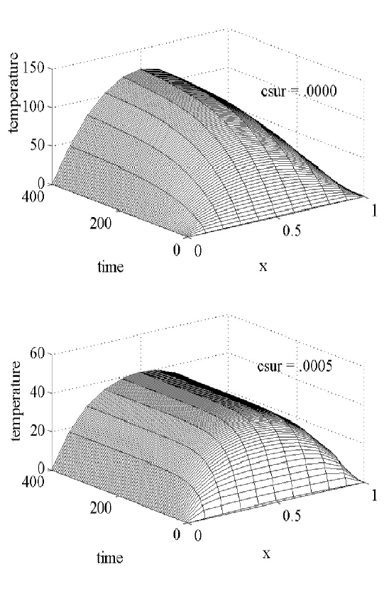
If one tries a calculation with
f
vxu
= =0005 with a time step size
equal to 5, then this violates the stability condition so that the model fails. For
f
vxu
=0005 the model did not fail with a final time equal to 400 and 100 time
steps so that the time step size equaled to 4. Note the maximum temperature
decreases from ab out 125 to about 40 as
f
vxu
increases from .0000 to .0005. In
order to consider larger
f
vxu
, the time step may have to be decreased so that
the stability condition will be satisfied.
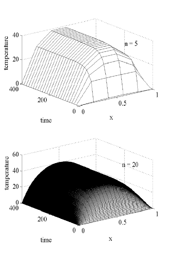
In the next numerical experiment we vary the number of space steps from
q = 10 to q = 5 and 20. This will change the k = g{, and we will have to
adjust the time step so that the stability condition holds. Roughly, if we double
q, then we should quadruple the number of time steps. So, for q = 5 we will let
pd{n = 25, and for q = 20 we will l et pd{n = 400. The reader should check
the stability condition assuming the other parameters in the numerical model
are
x
vxu
= 10, f
vxu
= =0005, N = =001, = 1 and f = 1. Note the second
graph in Figure 1.3.1 where
q
1.3.6 Assessment
The heat conduction in a thin wire has a number of approximations. Dierent
mesh sizes in either the time or space variable will give di
erent numerical re-
sults. However, if the stability conditions hold and the mesh sizes decrease, then
the numerical computations will di
er by smaller amounts. Other variations
on the model include more complicated boundary conditions, variable thermal
properties and di
usion in more than one direction.
© 2004 by Chapman & Hall/CRC
Figure 1.3.1.
= 10 and those in Figure 1.3.2 are similar.
22 CHAPTER 1. DISCRETE TIME-SPACE MODELS
Figure 1.3.1: Diusion in a Wire with csur = .0000 and .0005
© 2004 by Chapman & Hall/CRC
1.3. DIFFUSION IN A WIRE WITH LITTLE INSULATION 23
Figure 1.3.2: Diusion in a Wire with n = 5 and 20
© 2004 by Chapman & Hall/CRC
24 CHAPTER 1. DISCRETE TIME-SPACE MODELS
The above discrete model will converge, under suitable conditions, to a
continuum model of heat di
usion. This is a partial dierential equation with
initial and boundary conditions similar to those in (1.3.3), (1.3.4) and (1.3.5):
fx
w
= i + (Nx
{
)
{
+ f
vxu
(2@u)(x
vxu
x) (1.3.7)
x({> 0) = 0 and (1.3.8)
x(0> w) = 0 = x(O> w) (1.3.9)
The partial di
erential equation in (1.3.6) can be derived from (1.3.2) by re-
placing
x
n
l
by x(lk> nw), dividing by Dk w and letting k and w go to 0.
Convergence of the discrete model to the continuous model means for all
l and
n the errors
x
n
l
x(lk> nw)
go to zero as
k and w go to zero. Because partial dierential equations are
often impossible to solve exactly, the discrete models are often used.
Not all numerical methods have stability constraints on the time step. Con-
sider (1.3.6) and use an implicit time discretization to generate a sequence of
ordinary di
erential equations
f(x
n+1
x
n
)@w = i + (Nx
n+1
{
)
{
+ f
vxu
(2@u)(x
vxu
x
n+1
)= (1.3.10)
This does not have a stability constraint on the time step, but at each time step
one must solve an ordinary di
erential equation with boundary conditions. The
numerical solution of these will be discussed in the following chapters.
1.3.7 Exercises
1.
e!cient. Furthermore, use f
vxu
= =0002 and =0010.
2. In heat1d.m exp eriment with di
erent surrounding t emperatures x
vxu
=
5> 10> 20.
3. Suppose the surrounding temperature starts at -10 and increases by one
degree every ten units of time.
(a). Modify the finite di
erence model (1.3.3) is account for this.
(b). Modify the M
AT LAB code heat1d.m. How does this change the
long run solution?
4. Vary the
u = =01> =02> =05 and =10. Explain your computed results. Is this
model realistic for "large" u?
5. Verify equation (1.3.3) by using equation (1.3.2).
6. Consider the 3 × 3
D matrix version of line (1.3.3) and the example of
the stability condition on the time s tep. Observe D
n
for n = 10> 100 and 1000
with di
erent values of the time step so that the stability condition either does
or does not hold.
7. Consider the finite di
erence mo del with q = 5 so that there are four
unknowns.
© 2004 by Chapman & Hall/CRC
Duplicate the computations in Figure 1.3.1 with variable insulation co-
1.4. FLOW AND DECAY OF A POLLUTANT IN A STREAM 25
(a). Find 4 × 4 matrix version of (1.3.3).
(b). Repeat problem 6 with this 4 × 4 matrix
8. Experiment with variable space steps
k = g{ = O@q by letting q =
5
> 10> 20 and 40.
steps so that the stability condition holds.
9. Experiment with variable time steps
gw = W@pd{n by letting pd{n =
100> 200 and 400 with q = 10 and W = 400.
10. Examine the graphical output from the experiments in exercises 8 and
9. What happens to the numerical solutions as the time and space step sizes
decrease?
11. Suppose the thermal conductivity is a linear function of the temp erature,
say,
N = frqg = =001 + =02x where x is the temperature.
(a). Modify the finite di
erence model in (1.3.3).
(b). Modify the M
AT LAB code heat1d.m to accommodate this variation.
Compare the numerical solution with those given in Figure 1.3.1.
1.4 Flow and Decay of a Pollutant in a Stream
1.4.1 Intro duction
Consider a river that has been polluted upstream. The concentration (amount
per volume) will decay and disperse downstream. We would like to predict at
any point in time and in space the concentration of the pollutant. The model
of the concentration will also have the form
x
n+1
= Dx
n
+e where the matrix D
will be defined by the finite dierence model, which will also require a stability
constraint on the time step.
1.4.2 Applied Area
Pollution levels in streams, lakes and underground aquifers have become very
serious common concern. It is important to be able to understand the conse-
quences of possible pollution and to be able to make accurate predictions ab out
"spills" and future "environmental" policy.
Perhaps, the simplest model for chemical pollution is based on chemical
decay, and one model is similar to radioactive decay. A continuous model is
x
w
= gx where g is a chemical decay rate and x = x(w) is the unknown
concentration. One can use Euler’s method to obtain a discrete version
x
n+1
=
x
n
+ w(g)x
n
where x
n
is an approximation of x(w) at w = nw, and stability
requires the following constraint on the time step 1
wg A 0.
Here we will introduce a second model where the pollutant changes location
because it is in a stream. Assume the concentration will depend on both space
and time. The space variable will only be in one direction, which corresponds
to the direction of flow in the stream. If the pollutant was in a deep lake, then
the concentration would depend on time and all three directions in space.
© 2004 by Chapman & Hall/CRC
See Figures 1.3.1 and 1.3.2 and be sure to adjust the time
26 CHAPTER 1. DISCRETE TIME-SPACE MODELS
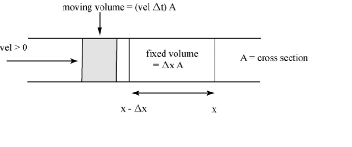
Figure 1.4.1: Polluted Stream
1.4.3 Model
Discretize both space and time, and let the concentration x at (l{> nw) be
approximated by
x
n
l
where w = W@pd{n> { = O@q and O is the length of the
stream. The model will have the general form
change in amount
(amount entering from upstream)
(amount leaving to downstream)
(amount decaying in a time interval)=
This is depicted in Figure 1.4.1 where the steam is moving from left to right and
the stream velocity is positive. For time we can choose either nw ru (n + 1)w.
Here we will choose
nw and this will eventually result in the matrix version of
the first order finite di
erence method.
Assume the stream is moving from left to right so that the stream velocity is
positive, yho A 0. Let D be the cross sectional area of the stream. The amount
of pollutant entering the left side of the volume
D{ (yho A 0) is
D(w yho) x
n
l
1
.
The amount leaving the right side of the volume
D{ (yho A 0)is
D(w yho) x
n
l
=
Therefore, the change in the amount from the stream’s velocity is
D(w yho) x
n
l
1
D(w yho) x
n
l
.
The amount of the pollutant in the volume
D{ at time nw is
D{ x
n
l
.
© 2004 by Chapman & Hall/CRC