Vidakovic B. Statistics for Bioengineering Sciences: With Matlab and WinBugs Support

Подождите немного. Документ загружается.

136 5 Random Variables

strength of heartbeat, and reﬂex, with a high score indicating a healthy infant.

Let the random variable X denote the Apgar score of a randomly selected new-

born infant at a particular hospital. Suppose that X has a given probability

distribution:

0 1 2 3 4 5 6 7 8 9 10

Prob .002 .001 .002 .005 .02 .04 .17 .38 .25 .12 .01

The following MATLAB program calculates (a)

EX , (b) Var (X ), (c) EX

, (d)

F(x), (e)

P(X <4), and (f) P (2 < X ≤3):

X = 0:10;

p = [0.002 0.001 0.002 0.005 0.02 ...

0.04 0.17 0.38 0.25 0.12 0.01];

EX = X

p’ %(a) EX = 7.1600

VarX = (X-EX).^2

p’ %(b) VarX = 1.5684

EX4 = X.^4

p’ %(c) EX4 = 3.0746e+003

ps = [0 cumsum(p)];

Fx = @(x) ps( min(max( floor(x)+2, 1),12) ); %handle

Fx(3.45) %(d) ans = 0.0100

sum(p(X < 4)) %(e) ans = 0.0100

sum(p(X > 2 & X <= 3)) %(f) ans = 0.0050

Note that the CDF F is expressed as function handle Fx to a custom-made

function.

Example 5.3. Cells. Randomly observed circular cells on a plate have a diam-

eter D that is a random variable with the following PMF:

8 12 16

Prob 0.4 0.3 0.3

(a) Find the CDF for D.

(b) Find the PMF for the random variable A

= D

π/4 (the area of a cell).

Show that

EA 6=(ED)

π/4. Explain.

Var (A).

(d) Find the moment-generating functions m

(t) and m

(t). Find Var (A)

using its moment-generating function.

(e) It is known that a cell with D

> 8 is observed. Find the probability of

=12 taking into account this information.

Solution:

(a)

(d) =











0, d <8

0.4, 8

≤ d <12

0.7, 12

≤ d <16

1, d

≥16

(b)

5.2 Discrete Random Variables 137

A 8

π/4 12

π/4 16

π/4

Prob 0.4 0.3 0.3

16π 36π 64 π

Prob 0.4 0.3 0.3

EA =16 π(

) +36π(

) +64π(

) =

364π

=114.3540.

ED =8(

) +12(

) +16(

) =116/10 =11.6

(ED)

3364π

100

364π

The expectation is a linear operator, and such a “plug-in” operation would

work only if the random variable A were a linear function of D, i.e., if A

αD +β, E A = αED +β. In our case, A is quadratic in D, and “passing” the

expectation through the equation is not valid.

(c)

Var A =EA

−(E A)

=1720π

−1324.96 π

=395.04π

since

Prob 0.4 0.3 0.3

(e) When D

>8 is true, only two values for D are possible, 12 and 16. These

values are equally likely. Thus, the distribution for D

|{D >8} is

|{D >8} 12 16

Prob 0.3/0.6 0.3/0.6

and

P(D = 12|D > 8) = 1/2. We divided 0.3 by 0.6 since P (D > 8) = 0.6. From

the deﬁnition of the conditional probability it follows that,

P(D = 12| D > 8) =

(D =12, D >8)/P(D >8) =P(D =12)/P(D >8) =0.3/0.6 =1/2.

There are important properties of discrete distributions in which the real-

izations x

, x

,... , x

are irrelevant and the focus is on the probabilities only,

for example, the measure of entropy. For a discrete random variable where the

probabilities are p

=(p

, p

,... , p

) the (Shannon) entropy is deﬁned as

H (p) =−

log(p

Entropy is a measure of the uncertainty of a random variable and for ﬁnite

discrete distributions achieves its maximum when the probabilities of realiza-

tions are equal, p

=(1/n,1/n,...,1/n).

For the distribution in Example 5.2, the entropy is 1.5812.

and E A

=1720π

(d)

(

)

12t

16t

and

(

)

16πt

0.3e

36πt

+0.3e

64πt

From m

(t) =6.4e

16πt

+10.8e

36πt

+19.2e

64πt

, and m

(t) =6.4e

16πt

+10.8e

36πt

19.2e

64πt

, we ﬁnd m

(0) = 36.4π and m

(0) = 1720π, leading to the result in

(c).

138 5 Random Variables

ps = [.002 .001 .002 .005 .02 .04 .17 .38 .25 .12 .01]

entropy = @(p) -sum( p(p>0) .

log(p(p>0)))

entropy(ps) %1.5812

The maximum entropy for distributions with 11 possible realizations is 2.3979.

5.2.1 Jointly Distributed Discrete Random Variables

So far we have discussed probability distributions of a single random vari-

able. As we delve deeper into this subject, a two-dimensional extension will be

needed.

When two or more random variables constitute the coordinates of a random

vector, their joint distribution is often of interest. For a random vector (X ,Y )

the joint distribution function is deﬁned via the probability of the event

{X ≤

x,Y ≤ y},

F(x, y)

=P(X ≤ x,Y ≤ y).

The univariate case

P(a ≤ X ≤ b) = F(b)−F(a) takes the bivariate form

P(a

≤ X ≤ a

, b

≤Y ≤ b

) = F(a

, b

) −F(a

, b

) −F(a

, b

) +F(a

, b

Marginal CDFs F

and F

are deﬁned as follows: for X , F

(x) = F(x, ∞)

and for Y as F

(y) = F(∞, y).

For a discrete bivariate random variable, the PMF is

p(x, y)

=P(X = x,Y = y),

x,y

p(x, y) =1,

while for marginal random variables X and Y the PMFs are

(x) =

p(x, y), p

(y) =

p(x, y).

The conditional distribution of X given Y

= y is deﬁned as

X |Y =y

(x) = p(x, y)/p

(y),

and, similarly, the conditional distribution for Y given X

= x is

Y |X =x

(y) = p(x, y)/p

(x).

When X and Y are independent, for any “cell” (x, y), p(x, y)

=P(X = x, Y =

y) = P(X = x)P(Y = y) = p

(x) p

(y), that is, the joint probability of (x, y)

is equal to the product of the marginal probabilities. If, on the other hand,

5.2 Discrete Random Variables 139

p(x, y) = p

(x)p

(y) holds for every (x, y), then X and Y are independent. The

independence of two discrete random variables is fundamental for the infer-

ence in contingency tables (Chap. 14) and will be revisited later.

Example 5.4. The PMF of a two-dimensional discrete random variable is given

by the following table:

5 10 15

0.1 0.2 0.3

0.25 0.1 0.05

The marginal distributions for X and Y are

1 2

Prob 0.6 0.4

and

5 10 15

Prob 0.35 0.3 0.35

while the conditional distribution for X when Y

=10 and the conditional dis-

tribution for Y when X

=2 are

|Y =10 1 2

Prob 0.2/0.3 0.1/0.3

and

|X =2 5 10 15

Prob 0.25/0.4 0.1/0.4 0.05/0.4

respectively.

Here X and Y are not independent since

0.1

=P(X =1,Y =5) 6=P(X =1)P (Y =5) =0.6 ·0.35 =0.21.

For two independent random variables X and Y , EX Y = EX ·EY , that is,

the expectation of a product of random variables is equal to the product of

their expectations.

The covariance of two random variables X and Y is deﬁned as

Cov(X ,Y ) =E((X −EX ) ·(Y −EY )) =EX Y −EX ·EY .

For a discrete random vector (X ,Y ),

EX Y =

xyp(x, y), and the covari-

ance is expressed as

Cov(X ,Y ) =

xyp(x, y) −

(x)

(y).

It is easy to see that the covariance satisﬁes the following properties:

140 5 Random Variables

Cov(X , X) =Var (X ),

Cov(X ,Y ) =Cov(Y , X), and

Cov(aX +bY , Z) = a Cov(X , Z) +b Cov(Y , Z).

For (X ,Y ) from Example 5.4 the covariance between X and Y is

−1. The

calculation is provided in the following MATLAB code. Note that the distribu-

tion of the product X Y is found in order to calculate

EX Y .

X=[1 2]; pX=[0.6 0.4]; EX = X

pX’

%EX = 1.4000

Y=[5 10 15]; pY=[0.35 0.3 0.35]; EY = Y

pY’

%EY =10

XY =[5 10 15 20 30];

pXY=[0.1 0.2+0.25 0.3 0.1 0.05]; EXY=XY

pXY’

%EXY = 13

CovXY = EXY - EX

%CovXY = -1

The correlation between random variables X and Y is the covariance nor-

malized by the standard deviations:

Corr(X ,Y ) =

ov(X ,Y )

Var X ·Var Y

In Example 5.4, the variances of X and Y are

Var X =0.24 and Var Y = 17.5.

Using these values, the correlation

Corr(X ,Y ) is −1/

0.24 ·17.5 = −0.488.

Thus, the random components in (X ,Y ) are negatively correlated.

5.3 Some Standard Discrete Distributions

5.3.1 Discrete Uniform Distribution

A random variable X that takes values from 1 to n with equal probabilities

of 1/n is called a discrete uniform random variable. In MATLAB

unidpdf and

unidcdf are the PDF and CDF of X , while unidinv is its quantile. For example,

unidpdf(1:5, 5)

%ans = 0.2000 0.2000 0.2000 0.2000 0.2000

unidcdf(1:5, 5)

%ans = 0.2000 0.4000 0.6000 0.8000 1.0000

are the PDF and CDF of the discrete uniform distribution on {1, 2,3,4,5}. From

i = n(n +1)/2, and

= n(n +1)(2n +1)/6 one can derive EX = (n +

5.3 Some Standard Discrete Distributions 141

1)/2 and Var X = (n

−1)/12. One of the important uses of discrete uniform

distribution is in nonparametric statistics (p. 482).

Example 5.5. Discrete Uniform: A Basis for Random Sampling. Suppose

that a population is ﬁnite and that we need a sample such that every subject

in the population has an equal chance of being selected.

If the population size is N and a sample of size n is needed, then if replace-

ment is allowed (each sampled object is recorded and then returned back to

the population), there would be N

possible equally likely samples. If replace-

ment is not allowed or possible (all subjects in the selected sample are to be

different, that is, sampling is without replacement), then there would be

different equally likely samples (see Sect. 3.5 for a deﬁnition of

The theoretical model for random sampling is the discrete uniform distri-

bution. If replacement is allowed, each of

{1,2,.. . , N} has a probability of 1/N

of being selected. In the case of no replacement, possible subsets of n subjects

can be indexed as

{1,2,.. . ,

}

and each subset has a probability of 1/

being selected.

In MATLAB, random sampling is achieved by the function

randsample. If

the population has n indexed subjects (from 1 to n), the indices in a random

sample of size k are found as

indices=randsample(n,k).

If it is possible to code the entire population as a vector

population, then

taking a sample of size k is done by

y=randsample(population,k).

The default is set to sampling without replacement. For sampling with

replacement, the ﬂag for replacement should be

’true’. If the sampling is done

with replacement, it can be weighted with a nonnegative weight assigned to

each subject in the population:

y=randsample(population,k,true,w). The size

of weight vector

w should be the same as that of population.

For instance,

randsample([’A’ ’C’ ’G’ ’T’],50,true,[1 1.5 1.4 0.9])

%ans = GCCTAGGGCATCCAAGTCGCGGCCGAGAATCAACGTTGCAGTGCTCAAAT

5.3.2 Bernoulli and Binomial Distributions

A simple Bernoulli random variable Y is dichotomous with P(Y = 1) = p and

P(Y = 0) = 1 − p for some 0 ≤ p ≤1 and is denoted as Y ∼ B er(p). It is named

after Jakob Bernoulli (1654–1705) a prominent Swiss mathematician and as-

tronomer (Fig. 5.3a). Suppose that an experiment consists of n independent

trials (Y

,... , Y

) in which two outcomes are possible (e.g., success or failure),

with

P(success) =P(Y =1) = p for each trial. If X = x is deﬁned as the number

of successes (out of n), then X

+···+Y

and there are

arrangements

of x successes and n

−x failures, each having the same probability p

(1−p)

n−x

X is a binomial random variable with the PMF

142 5 Random Variables

(x) =

(1 − p)

n−x

, x =0,1,..., n.

This is denoted by X

∼ B in(n, p). From the moment-generating function

(t) =(pe

+(1 − p))

we obtain µ =EX = n p and σ

=Var X = np(1− p).

The cumulative distribution for a binomial random variable is not simpli-

ﬁed beyond the sum, i.e., F(x)

i≤x

(i). However, interval probabilities can

be computed in MATLAB using

binocdf(x,n,p), which computes the CDF at

value x. The PMF can also be computed in MATLAB using

binopdf(x,n,p). In

WinBUGS, the binomial distribution is denoted as

dbin(p,n). Note the oppo-

site order of parameters n and p.

Example 5.6. Left-Handed Families. About 10% of the world’s population is

left-handed. Left-handedness is more prevalent in men (1/9) than in women

(1/13). Studies have shown that left-handedness is linked to the gene LR-

RTM1, which affects the symmetry of the brain. In addition to its genetic

origins, left-handedness also has developmental origins. When both parents

are left-handed, a child has a probability of 0.26 of being left-handed.

Ten families in which both parents are left-handed and have a single child

are selected, and the ten children are inspected for left-handedness. Let X be

the number of left-handed among the inspected. What is the probability that

(a) Is equal to 3?

(b) Falls anywhere between 3 and 6, inclusive?

(d) Is not less than 4?

(e) Would you be surprised if the number of left-handed children among

the ten inspected was eight? Why or why not?

The solution is given by the following annotated MATLAB script.

% Solution

disp(’(a) Bin(10, 0.26): P(X = 3)’);

binopdf(3, 10, 0.26)

% ans = 0.2563

disp(’(b) Bin(10, 0.26): P(3 <= X <= 6)’);

% using binopdf(x, n, p)

disp(’(b)-using PDF’); binopdf(3, 10, 0.26) + ...

binopdf(4, 10, 0.26) + binopdf(5, 10, 0.26)+ binopdf(6, 10, 0.26)

% using binocdf(x, n, p)

disp(’(b)-using CDF’); binocdf(6, 10, 0.26) - binocdf(2, 10, 0.26)

% ans = 0.4998

%(c) at most four i.e., X <= 4

disp(’(c) Bin(10, 0.26): P(X <= 4)’); binocdf(4, 10, 0.26)

% ans = 0.9096

%(d) not less than 4 is 4,5,...,10, or complement of <=3

disp(’(d) Bin(12, 0.7): P(X >= 4)’); 1-binocdf(3, 10, 0.26)

% ans = 0.2479

disp(’(e) Bin(10, 0.26): P(X = 8)’);

5.3 Some Standard Discrete Distributions 143

binopdf(8, 10, 0.26)

% ans = 5.1459e-004

% Yes, this is a surprising outcome since the probability

% of this event is rather small, 0.0005.

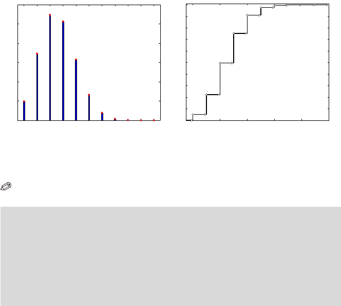
Panels (a) and (b) in Fig. 5.2 show respectively the PMF and CDF for the

binomial

B in(10,0.26) distribution.

0 1 2 3 4 5 6 7 8 9 10

0.05

0.1

0.15

0.2

0.25

0 2 4 6 8 10

0.1

0.2

0.3

0.4

0.5

0.6

0.7

0.8

0.9

(a) (b)

Fig. 5.2 Binomial

B in(10,0.26) (a) PMF and (b) CDF.

How does one recognize that random variable X has a binomial distri-

bution?

(a) It allows an interpretation as the sum of “successes” in n Bernoulli

trials, for n ﬁxed.

(b) The Bernoulli trials are independent.

Next we discuss how to deal with a binomial-like framework in which con-

dition (c) is violated.

Generalized Binomial Sampling*. Suppose that n independent experi-

ments are performed and that an event A has a probability of p

of appearing

in the ith experiment.

We are interested in the probability that A appeared exactly k times in

the n experiments. The binomial setup is not directly applicable since the

probabilities of A differ from experiment to experiment. However, the bi-

nomial setup is useful as a hint on how to solve the general case. In the

binomial setup the probability of k events A in n experiments is equal to

144 5 Random Variables

the coefﬁcient of z

in the expansion of G(z) = (pz + q)

. Indeed, (pz + q)

+···+

n−k

+···+n pq

n−1

z + p



The polynomial G(z) is called the probability-generating function. If X

is a discrete integer-valued random variable such that p

=P(X = n), then its

probability-generating function is deﬁned as

(z) =Ez

Note that in the polynomial G

(z), the probability p

=P(X = n) is the coefﬁ-

cient of the power z

. Also, G

) is the moment-generating function m

(z).

In the general binomial setup, the polynomial (pz

+q)

becomes

(z) =(p

z +q

) ×(p

z +q

) ×···×(p

z +q

) =

i=0

(5.5)

and the probability that there are k events A in n experiments is equal to

the coefﬁcient a

of z

in the polynomial G

(z). This follows from the two

properties of G(z): (i) When X and Y are independent, G

X +Y

(z) =G

(z) G

(z),

and (ii) if X is a Bernoulli

B er(p), then G

(z) = pz +q.

Example 5.7. System with Unreliable Components. Let S be a system

consisting of ten unreliable components that work and fail independently of

each other. The components are operational in some ﬁxed time interval [0,T]

with the probabilities

ps =[0.5 0.3 0.2 0.5 0.6 0.4 0.2 0.4 0.7 0.8];

Let a random variable X represent the number of components that remain

operational after time T.

Find (a) the distribution for X and (b)

EX and Var X.

ps =[0.5 0.3 0.2 0.5 0.6 0.4 0.2 0.4 0.7 0.8];

qs = 1- ps;

all = [ps’ qs’];

[m n]= size(all);

Gz = [1]; %initial

for i = 1:m

Gz = conv(Gz, all(i,:) );

% conv as polynomial multiplication

end

%at the end, Gz is the product of p

i x + q

sum(Gz) %the sum is 1

probs = Gz(end:-1:1);

k = 0:10

% probs=[0.0010 0.0117 0.0578 0.1547 0.2507 ...

% 0.2582 0.1716 0.0727 0.0188 0.0027 0.0002]

EX = k

probs’ %expectation 4.6

EX2 = k.^2

probs’;

VX = EX2 - (EX)^2 %variance 2.12

5.3 Some Standard Discrete Distributions 145

Note that in the above script we used the convolution operation conv to

multiply polynomials, as in

conv([2 -1],[1 3 2])

% ans = 2 5 1 -2,

which is interpreted as (2z −1) ·(z

+3z +2) =2z

+5z

+z −2.

From the MATLAB calculations we ﬁnd that the probability-generating

function G(z) from (5.5) is

G(z)

= 0.00016128z

+0.00268992z

+0.01883264z

+0.07273456z

0.17155808z

+0.25816544z

+0.25070848z

+0.15470576z

0.05777184z

+0.01170432z +0.00096768,

and the random variable X , the number of operational items, has the following

distribution (after rounding to four decimal places):

X 0 1 2 3 4 5 6 7 8 9 10

Prob 0.0010 0.0117 0.0578 0.1547 0.2507 0.2582 0.1716 0.0727 0.0188 0.0027 0.0002

The answers to (b) are EX =4.6 and Var X =2.12.

Note that a “solution” in which one ﬁnds the average of the component

probabilities,

ps, as

p =

(0.5 +0.3 +···+0.8) = 0.46, and then applies the

standard binomial calculation will lead to the correct expectation, 4.6, because

of linearity. However, the variance and probabilities for X would be different.

For example, the probability

P(X = 4) would be binopdf(4,10,0.46)=0.2331,

while the correct value is 0.2507.

(a) (b)

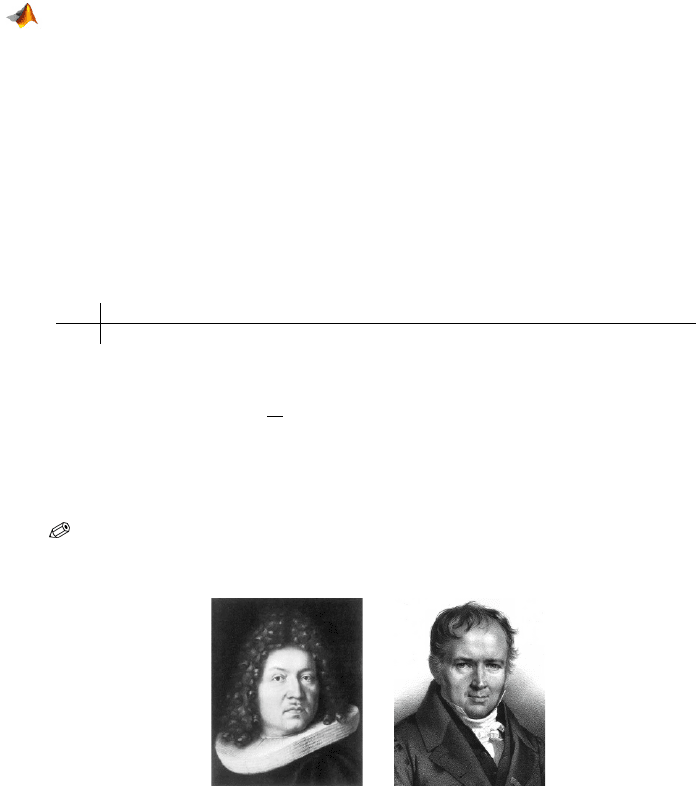
Fig. 5.3 (a) Jacob Bernoulli (1654–1705), Swiss mathematician and astronomer. His mono-

graph Ars Conjectandi, published posthumously in 1713, contains his explorations in prob-

ability theory, states a form of the law of large numbers, and describes experiments that

we call now Bernoulli trials. (b) Siméon Denis Poisson (1781–1840), French mathematician

and physicist. His book Recherches sur la probabilité des jugements en matières criminelles

et matière civile, published in 1837, applies probability theory to the decisions of juries. It

introduces a discrete probability distribution, now known as the Poisson distribution.