Vidakovic B. Statistics for Bioengineering Sciences: With Matlab and WinBugs Support

Подождите немного. Документ загружается.

156 5 Random Variables

% is the same as

binopdf(5, 5+15, 0.6)

%ans = 0.0013

Example 5.15. Suppose that the probabilities of blood groups in a particular

population are given as

O A B AB

0.37 0.39 0.18 0.06

If eight subjects are selected at random from this population, what is the

probability that

(a) (O, A,B, AB)

=(3,4,1,0)?

(b) O

=5?

In (a), the probability is

factorial(8) /(factorial(3)

...

factorial(4)

factorial(1)

factorial(0))

...

0.37^3

0.39^4

0.18^1

0.06^0

%ans = 0.0591

%or

mnpdf([3 4 1 0],[0.37 0.39 0.18 0.06])

%ans = 0.0591.

In (b), O ∼B in(8,0.37) and P(O =3) =0.2815.

5.3.8 Quantiles

Quantiles of random variables are deﬁned as follows. A p-quantile (or 100 × p

percentile) of random variable X is the value x for which F(x)

= p, where F is

the cumulative distribution function for X . For discrete random variables this

deﬁnition is not unique and modiﬁcation is needed:

F(x)

=P(X ≤ x) ≥ p and P(X ≥ x) ≥1 − p.

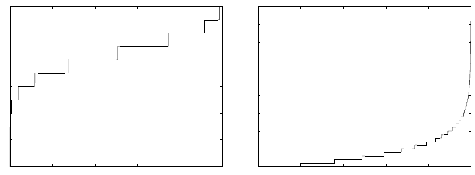
For example, the 0.05 quantile of a binomial distribution with parameters

= 12 and p = 0.7 is x = 6 since P(X ≤ 6) = 0.1178 ≥ 0.05 and P(X ≥ 6) =

1 −P(X ≤5) =1 −0.0386 =0.9614 ≥ 0.95. Binomial B in(12,0.7) and geometric

G (0.2) quantiles are shown in Fig. 5.7.

quab =[]; quag =[];

for p = 0.00:0.0001:1

quab = [quab binoinv(p, 12, 0.7)];

quag = [quag geoinv(p, 0.2)];

end

figure(1)

5.4 Continuous Random Variables 157

plot([0.00:0.0001:1],quab,’k-’)

figure(2)

plot([0.00:0.0001:1],quag,’k-’)

0 0.2 0.4 0.6 0.8 1

(a) (b)

Fig. 5.7 (a) Binomial

B in(12,0.7) and (b) geometric G (0.2) quantiles.

5.4 Continuous Random Variables

Continuous random variables take values within an interval (a, b) on a real

line R. The probability density function (PDF) f (x) fully speciﬁes the variable.

The PDF is nonnegative, f (x)

≥ 0, and integrates to 1,

f (x) dx = 1. The

probability that X takes a value in an interval (a, b) (and for continuous r.v.

equivalently [a, b),(a,b], or [a,b]) is

P[X ∈(a, b)] =

f (x)dx.

The CDF is

F(x)

=P(X ≤ x) =

−∞

f (t)dt.

In terms of the CDF,

P[X ∈(a, b)] =F(b) −F(a).

The expectation of X is given by

EX =

x f (x)dx.

The expectation of a function of a random variable g(X ) is

Eg(X ) =

g(x)f (x)dx.

The kth moment of a continuous random variable X is deﬁned as

f (x)dx, and the kth central moment is E(X −EX )

(x−EX )

f (x)dx. As

158 5 Random Variables

in the discrete case, the ﬁrst moment is the expectation and the second central

moment is the variance,

(X ) =E(X −EX )

The moment-generating function of a continuous random variable X is

m(t)

=Ee

f (x)dx.

Since m

(k)

(t) =

f (x)dx, EX

= m

(k)

(0).

Moment-generating functions are related to Laplace transforms of densi-

ties. Since the bilateral Laplace transform of f (x) is deﬁned as

L (f ) =

−tx

f (x)dx,

it holds that m(

−t) =L (f ).

The entropy of a continuous random variable with a density f (x) is deﬁned

H (X ) =−

f (x)log f (x)dx

whenever this integral exists. Unlike the entropy for discrete random vari-

ables,

H (X ) can be negative and not necessarily invariant with respect to a

transformation of X .

Example 5.16. Markov’s Inequality. If X is a random variable that takes

only nonnegative values, then for any positive constant a

P(X ≥ a) ≤

. (5.8)

Indeed,

EX =

∞

x f (x)dx ≥

∞

x f (x)dx ≥

∞

a f (x)dx = a

∞

f (x)dx = aP(X ≥a).

An average mass of a single cell of E. coli bacterium is 665 fg (femtogram,

fg=10

−15

g). If a particular cell of E. coli is inspected, what can be said about

the probability that its weight will exceed 1000 fg? According to Markov’s in-

equality, this probability does not exceed 665/1000 = 0.665.

5.4.1 Joint Distribution of Two Continuous Random

Variables

Two random variables X and Y are jointly continuous if there exists a non-

negative function f (x, y) so that for any two-dimensional domain D,

5.4 Continuous Random Variables 159

P((X ,Y ) ∈ D) =

Z Z

f (x, y)dxd y.

When such a two-dimensional density f (x, y) exists, it is a repeated partial

derivative of the cumulative distribution function F(x, y)

=P(X ≤ x,Y ≤ y),

f (x, y)

∂

F(x, y)

∂x ∂y

The marginal densities for X and Y are, respectively, f

(x) =

∞

−∞

f (x, y)d y

and f

(y) =

∞

−∞

f (x, y)dx. The conditional distributions of X when Y = y and

of Y when X

= x are

f (x

|y) = f (x, y)/ f

(y) and f (y|x) = f (x, y)/f

(x).

The distributional analogy of the multiplication probability rule

P(AB) =

(A|B)P(B) = P(B|A)P(A) is

f (x, y)

= f (x|y)f

(y) = f (y|x)f

(x).

When X and Y are independent, the joint density is the product of marginal

densities, f (x, y)

= f

(x)f

(y). Conversely, if the joint density of (X ,Y ) can be

represented as a product of marginal densities, X and Y are independent.

The deﬁnition of covariance and the correlation for X and Y coincides with

the discrete case equivalents:

Cov(X ,Y ) =EX Y −EX ·EY and Corr(X ,Y ) =

ov(X ,Y )

Var (X )·Var (Y )

Here,

EX Y =

xyf (x, y)dxd y.

valve is one of the oldest cardiac valve prostheses in the world. The ﬁrst aortic

valve replacement (AVR) with a Starr–Edwards metal cage and silicone ball

valve was performed in 1961. Follow-up studies have documented the excellent

durability of the Starr–Edwards valve as an AVR. Suppose that the durability

of the Starr–Edwards valve (in years) is a random variable X with density

f (x)







/100, 0 < x <10,

a(x

−30)

/400, 10 ≤ x ≤30,

0, otherwise.

(a) Find the constant a.

(b) Find the CDF F(x) and sketch graphs of f and F.

ance.

Solution: (a) Since 1

f (x)dx,

Example 5.17. Durability of the Starr–Edwards Valve. The Starr–Edwards

160 5 Random Variables

1 =

/100dx +

a(x −30)

/400dx = ax

/300 |

+a(x −30)

/1200 |

This gives 1000a/300

−0 +0 −(−20)

a/1200 =10a/3 +20a/3 = 10a = 1, that is,

=1/10. The density is

f (x)







/1000, 0 < x <10,

−30)

/4000, 10 ≤ x ≤30,

0, otherwise.

(b) The CDF is

F(x)











0, x <0,

/3000, 0 < x <10,

+(x −30)

/12000, 10 ≤ x ≤30,

1, x

≥30.

+(x−30)

/12000 =0.6 and

is x

=13.131313.... The mean is EX =25/2, and the 60th percentile exceeds the

mean. E X

=180, thus the variance is Var X =180 −(25/2)

=95/4 =23.75.

Example 5.18. A two-dimensional random variable (X , Y ) is deﬁned by its den-

sity function, f (x, y)

=2xe

−x−2y

, x ≥0, y ≥0.

(a) Find the probability that random variable (X , Y ) falls in the rectangle

≤ X ≤1,1 ≤Y ≤2.

(b) Find the marginal distributions of X and Y .

|{Y = y} Does it depend on y?

Solution: (a) The joint density separates variables x and y, therefore

P(0 ≤ X ≤1, 1 ≤Y ≤2) =

−x

dx ×

−2y

d y.

Since

−x

dx =−xe

−x

dx =−e

−1

−e

−1

+1 =1 −2/e,

and

−2y

d y =−e

−2y

=−e

−4

−2

−1

then

P(0 ≤ X ≤1, 1 ≤Y ≤2) =

e −2

−1

≈0.0309.

5.5 Some Standard Continuous Distributions 161

(b) Since the joint density separates the variables, it is a product of

marginal densities f (x, y)

= f

(x) × f

(y). This is an analytic way to state

that components X and Y are independent. Therefore, f

(x) = xe

−x

, x ≥ 0

and f

(y) =2e

, y ≥0.

|{Y = y} and Y |{X = x} are deﬁned as

f (x

|y) = f (x, y)/ f

(y) and f (y|x) = f (x, y)/f

(x).

Because of independence of X and Y the conditional densities coincide with

the marginal densities. Thus, the conditional density for X

|{Y = y} does not

depend on y.

5.5 Some Standard Continuous Distributions

In this section we list some popular, commonly used continuous distributions:

uniform, exponential, gamma, inverse gamma, beta, double exponential, lo-

gistic, Weibull, Pareto, and Dirichlet. The normal (Gaussian) distribution will

be just brieﬂy mentioned here. Due to its importance, a separate chapter will

cover the details of the normal distribution and its close relatives:

, student

t, Cauchy, F, and lognormal distributions. Some other continuous distribu-

tions will be featured in the examples, exercises, and other chapters, such as

Maxwell and Rayleigh distributions.

5.5.1 Uniform Distribution

A random variable X has a uniform U (a, b) distribution if its density is given

(x) =

b−a

, a ≤ x ≤ b,

0, else .

Sometimes, to simplify notation, the density can be written simply as

(x) =

b −a

1(a ≤ x ≤ b).

Here,

1(A) is 1 if A is a true statement and 0 if A is false. Thus, for x < a or

> b, f

(x) =0, since 1(a ≤ x ≤ b) =0.

The CDF of X is given by

162 5 Random Variables

(x) =







0, x < a,

x−a

b−a

, a ≤ x ≤ b,

1, x

> b.

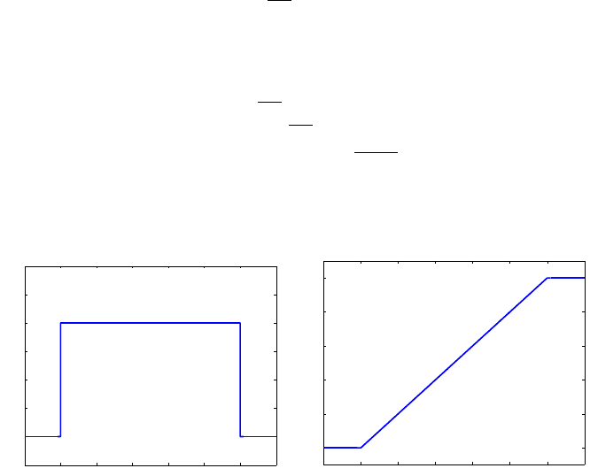
The graphs of the PDF and CDF of a uniform

U (−1, 4) random variable are

shown in Fig. 5.8.

For a

=0 and b =1, the distribution is called standard uniform.

If U is

U (0, 1), then X =−λlog(U) is an exponential random variable with

scale parameter

λ.

−2 −1 0 1 2 3 4 5

−0.05

0.05

0.1

0.15

0.2

0.25

−2 −1 0 1 2 3 4 5

0.2

0.4

0.6

0.8

(a) (b)

Fig. 5.8 (a) PDF and (b) CDF for uniform

U (−1,4) distribution. The graphs are plotted

as (a)

plot(-2:0.001:5, unifpdf(-2:0.001:5, -1, 4)) and (b) plot(-2:0.001:5,

unifcdf(-2:0.001:5, -1, 4))

The sum of two independent standard uniforms is triangular,

(x) =







x, 0 ≤ x ≤1,

−x, 1 ≤ x ≤2,

0, else .

This is sometimes called a “witch hat” distribution. The sum of n independent

standard uniforms is known as the Irwing–Hall distribution.

5.5.2 Exponential Distribution

The probability density function for an exponential random variable is

The expectation of X is

EX =

a+b

and the variance is Var X = (b −a)

/12.

The

th moment of

is given by

n+1

n−i

. The moment-generating

function for the uniform distribution is m(t)

−e

t(b−a)

5.5 Some Standard Continuous Distributions 163

(x) =

λe

−λx

, x ≥0,

0, else ,

where

λ >0 is called the rate parameter. An exponentially distributed random

variable X is denoted by X

∼ E (λ). Its moment-generating function is m(t) =

λ/(λ − t) for t < λ, and the mean and variance are 1/λ and 1/λ

, respectively.

The nth moment is

This distribution has several interesting features; for example, its failure

rate, deﬁned as

(t) =

(t)

1 −F

(t)

is constant and equal to

λ.

The exponential distribution has an important connection to the Poisson

distribution. Suppose we observe i.i.d. exponential variates (X

, X

,... ) and

deﬁne S

= X

+···+X

. For any positive value t, it can be shown that P(S

t < S

n+1

) = p

(n), where p

(n) is the probability mass function for a Poisson

random variable Y with parameter

λt.

Like a geometric random variable, an exponential random variable has the

memoryless property,

P(X ≥ u +v|X ≥ u) =P(X ≥v) (Exercise 5.17).

The median value, representing a typical observation, is roughly 70% of

the mean, showing how extreme values can affect the population mean. This

is explicitly shown by the ease in computing the inverse CDF:

=F(x) =1 −e

−λx

⇐⇒ x = F

−1

(p) =−

log(1 − p).

The MATLAB commands for exponential CDF, PDF, quantile, and ran-

dom number are

expcdf, exppdf, expinv, and exprnd. MATLAB uses the al-

ternative parametrization with 1/

λ in place of λ. Thus, the CDF of random

variable X with

E (3) distribution evaluated at x = 2 is calculated in MAT-

LAB as

expcdf(2,1/3). In WinBUGS, the exponential distribution is coded as

dexp(lambda).

Example 5.19. Melanoma. The 5-year cancer survival rate in the case of ma-

lignant melanoma of the skin at stage IIIA is 78%. Assume that the survival

time T can be modeled by an exponential random variable with unknown rate

λ.

Using the given survival rate of 0.78, we ﬁrst determine the parameter of

the exponential distribution – the rate

λ.

Since

P(T > t) = exp(−λt), P(T > 5) = 0.78 leads to exp{−5λ} = 0.78, with

solution

λ =−

log(0.78), which can be rounded to λ =0.05.

Next, we ﬁnd the probability that the survival time exceeds 10 years, ﬁrst

directly using the CDF,

P(T >10) =1 −F(10) =1 −

1 −e

−0.05·10

=0.6065,

164 5 Random Variables

and then by MATLAB. One should be careful when parameterizing the expo-

nential distribution in MATLAB. MATLAB uses the scale parameter, a recip-

rocal of the rate

λ.

1 - expcdf(10, 1/0.05)

%ans = 0.6065

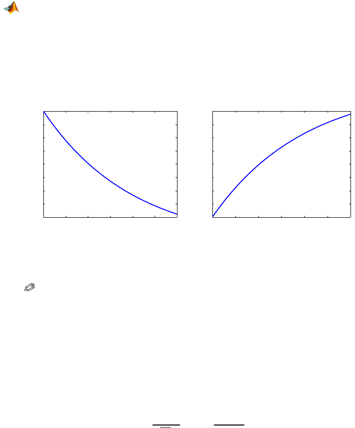
%Figures of PDF and CDF are produced by

time=0:0.001:30;

pdf = exppdf(time, 1/0.05); plot(time, pdf, ’b-’);

cdf = expcdf(time, 1/0.05); plot(time, cdf, ’b-’);

This is shown in Fig. 5.9.

0 5 10 15 20 25 30

0.01

0.015

0.02

0.025

0.03

0.035

0.04

0.045

0.05

Time (in years)

PDF

0 5 10 15 20 25 30

0.1

0.2

0.3

0.4

0.5

0.6

0.7

0.8

Time (in years)

CDF

(a) (b)

Fig. 5.9 Exponential (a) PDF and (b) CDF for rate

λ =0.05.

5.5.3 Normal Distribution

As indicated in the introduction, due to its importance, the normal distribu-

tion is covered in a separate chapter. Here we provide a deﬁnition and list a

few important facts. The probability density function for a normal (Gaussian)

random variable X is given by

(x) =

2π σ

exp

−

(x −µ)

2σ

where

µ is the mean and σ

is the variance of X . This will be denoted as

∼

For

µ = 0 and σ = 1, the distribution is called the standard normal dis-

tribution. The CDF of a normal distribution cannot be expressed in terms of

5.5 Some Standard Continuous Distributions 165

elementary functions and deﬁnes a function of its own. For the standard nor-

mal distribution the CDF is

Φ(x) =

−∞

2π

exp

−

dt.

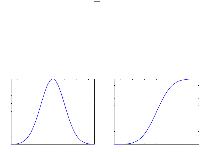
The standard normal PDF and CDF are shown in Fig. 5.10a,b.

The moment-generating function is m(t)

= exp{µt +σ

/2}. The odd cen-

tral moments

E(X −µ)

2k+1

are 0 because the normal distribution is symmetric

about the mean. The even moments are

E(X −µ)

=σ

(2k −1)!!,

where (2k

−1)!! =(2k −1) ·(2k −3)···5·3 ·1.

−3 −2 −1 0 1 2 3

0.05

0.1

0.15

0.2

0.25

0.3

0.35

PDF

−3 −2 −1 0 1 2 3

0.1

0.2

0.3

0.4

0.5

0.6

0.7

0.8

0.9

CDF

(a) (b)

Fig. 5.10 Standard normal (a) PDF and (b) CDF

Φ(x).

The MATLAB commands for normal CDF, PDF, quantile, and a random

number are

normcdf, normpdf, norminv, and normrnd. In WinBUGS, the normal

distribution is coded as

dnorm(mu,tau), where tau is a precision parameter, the

reciprocal of variance.

5.5.4 Gamma Distribution

The gamma distribution is an extension of the exponential distribution. Prior

to deﬁning its density, we deﬁne the gamma function that is critical in normal-

izing the density. Function

Γ(x) deﬁned via the integral

∞

x−1

−t

dt, x > 0

is called the gamma function (Fig. 5.11a). If n is a positive integer, then

Γ(n) =(n −1)!. In MATLAB: gamma(x).

Random variable X has a gamma

G a(r,λ) distribution if its PDF is given