Sundararaja D. The Discrete Fourier Transform. Theory, Algorithms and Applications

Подождите немного. Документ загружается.

184

DFT Algorithms for Real Data - II

The computational stages

There are m stages specified as r =

1,2,...,

m, where m = log

A stage

consists of Y butterflies. The expressions for the twiddle factor exponent

and the indices of the nodes of each group of butterflies are given, for

the first m

—

2 stages, (The butterflies of the last two stages and the first

butterfly of each group of butterflies of the other stages are special cases

and they will be explained later.) as follows.

h = imod2

, i =

0,1,...,

f - 1

(9 19)

I = h + 2

For example, with N = 32, there are 4 stages specified as r = 1,2,3, and

Four butterflies make up a stage. Indices h, I, and 11, and the twiddle

factor exponent s of each group of butterflies are given, respectively, by

h = i mod 2

(i = 0,1,2,3), / = h + 2

= 2

- h, and s = 2

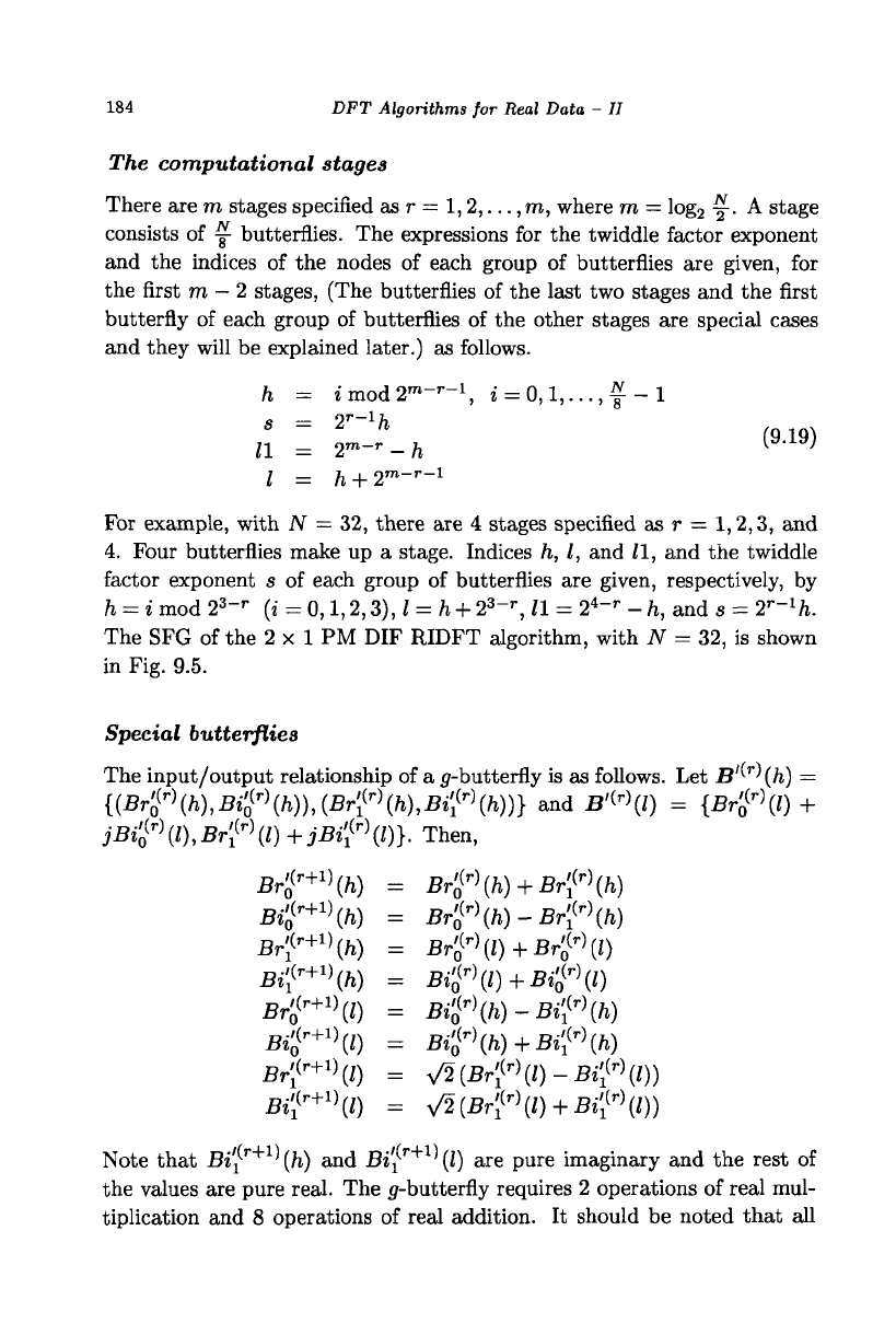
The SFG of the 2 x 1 PM DIF RIDFT algorithm, with N = 32, is shown

in Fig. 9.5.

Special butterflies

The input/output relationship of a p-butterfly is as follows. LetB'W(/i) =

{(Br$

Hh),B4

\h)),(Br'{

(h),Bi'i

\h))} and B'W(/) = {Br$

\l) +

jB4

(1),Br[

{r)

(I) + jBif

(I)}. Then,

Br'

{r+1

\h) = Br'

ir)

(h) + Br'!

\h)

Bi'

ir+1

\h) = B4

(h)-Br'l

\h)

Br'i

r+l)

(h) = B4

(l)+Br'

\l)

Bi'}

r+1

\h) = Bi$

\l) + Bi't

\l)

Br'

{r+1)

(l) = Bi'

\h)-Bi'l

\h)

Bi$

r+1

\l) = B4

(h)+Bi'i

\h)

Br'}

r+1

Hl) = V2(Br'}

(l)-Bi'}

\l))

Bi'}

r+1)

(l) = V2(Br'l

(l) + Bi'l

\l))

Note that Bi'£

r+1

\h) and Bi'{

r+1

'(l) are pure imaginary and the rest of

the values are pure real. The p-butterfly requires 2 operations of real mul-

tiplication and 8 operations of real addition. It should be noted that all

The 2 x 1 PM DIF RIDFT Algorithm 185

stage 1 stage 2 stage 3 stage 4

Fig. 9.5 The SFG of the 2 x 1 PM DIF RIDFT algorithm, with N = 32. Twiddle

factors are represented only by their exponents. For example, the number

—4

represents

the operations of this butterfly, except 4 additions, can be merged in the

twiddle factor computation of the preceding stage for about half the num-

ber of g—butterflies. The p-butterfly carries out the same processing, but

with reduced computation, that is carried out in the first and the middle

butterflies of each group of butterflies, up to the last but one stage, in the

corresponding DIF IDFT algorithm.

The input/output relationship of an /-butterfly is as follows. Let

B'^-

)^) = {(Br(,

(m_1)

(n)

Bi|f

(n)), (Bri

(n),B*

(rB_1)

(n))}.

Then,

Br'

(m)

(n) = flr(,

(,n

(n) + Br'

(n)

(n) = Br(,

(n)-Bri

(n)

Br'i

\n) = B»2

>(n)-£t'

(n)

Bi'}

\n) = S^

(n)+B<

(n)

The /-butterfly requires 4 operations of real addition and the computation

186

DFT Algorithms for Real Data - II

Vectors Stage 1 Stage 2 Stage 3 Stage 4

Output Output Output Swapped

Output

138.00

18.00

140.00

J4.00

4.78 + J22.67

-9.48 - jO.65

-31.11-j'14.0

20.91 -J27.02

-33.72-J16.4

-19.18 +J9.04

2+jO

14.14-j'14.14

-29.39 -

j'3.24

-5.19+J3.34

31.12+J14.00

-8.66 - j"23.44

-5.67 + J3.83

-19.89 -J32.29

156.00 120.00

4.00 jO.OO

-0.89 + J18.84

10.45 + j'26.50

0.01 - j/28.00

-62.23 - jO.OO

-63.11 -j'13.16

-4.33 - j/19.64

136.00

39.99

144.00

jO.OO

18.62+J23.32

-36.96 -J28.29

48.00 +J0.01

11.32-J33.93

-26.63 - jO.68

-15.31-j"5.60

160.0C

0.02

152.00

-J56.00

-64.00 +J32.00

62.22+J5.68

120.00

-88.01

120.00

-j'88.01

16.00+J40.00

-16.97 + J16.97

175.99

96.0C

96.01

J0.02

-8.01+^24.00

45.25+J22.64

144.0C

63.99

144.00

-J31.98

-24.00 - j'24.00

-22.63-J56.57

160.02

-128.0

208.00

79.96

31.99

32.00

208.0:

-48.0C

271.99

-16.05

95.9£

31.97

207.99

-48.0:

159.98

j'64.00

96.00

J96.03

208.01

J80.00

31.99

-jO.01

79.99

J48.0

96.03

j96.01

80.01

-J48.0

175.98 112.02

48.0C-jll2.01

32.02

95.98

255.97

31.99

64.00

128.01

159.98

128.00

287.96

-0.03

127.96

0.02

160.01

32.01

223.98

224.03

288.02

223.98

288.02

127.99

-0.01

288.00

256.00

32.01

128.04

192.03

64.01

192.04

256.01

31.98

127.99

0.00

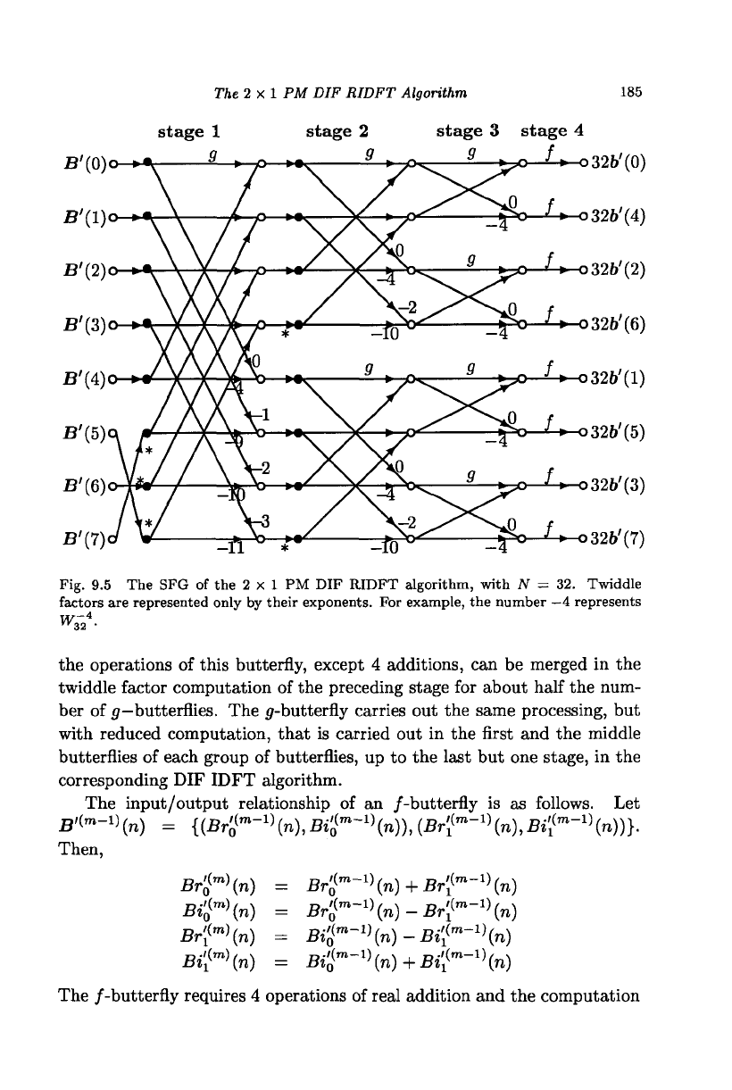
Fig. 9.6 The trace of the 2x1 PM DIF RIDFT algorithm, with N = 32.

is confined to the values of a single vector. The processing of this stage,

unscrambling of the output vectors, and dividing the output values by N

can be carried out at the same time to reduce the data transfer operations.

An /-butterfly carries out the same processing, but with reduced computa-

tion, that is carried out by a butterfly of the last stage in the corresponding

DIF IDFT algorithm.

Example 9.2 A trace table of the algorithm, shown in Fig. 9.5, is shown

in Fig. 9.6. Half of the DFT values are read into the storage locations of

8 vectors each consisting of two complex elements as shown in the last col-

umn of Fig. 9.3. The first column shows the values after vectors have been

formed. When a value is pure real or pure imaginary, it is shown separately

with a vertical line. The second, third, fourth, and fifth, columns show the

values, respectively, after the first, second, third, and fourth stage opera-

tions of the algorithm are carried out. Note that the swapping operation

is carried out along with the processing of stage 4. The output values have

to be divided by N = 32. Since the input data has been given only to a

precision of two digits, the output is not exact as expected. For example,

a;(0) = 32.02 instead of 32 in the last stage. Compare this table with that

given in Fig. 8.2 to find out how the redundancy at each stage is eliminated.

The

2 x 2 PM DIT

RDFT Algorithm

187

9.4

The 2x2 PM DIT

RDFT Algorithm

By merging

the

multiplication operations

adjacent stages

of the 2x1

DIT

RDFT algorithm,

obtain

the 2 x 2 PM DIT

RDFT algorithm.

The

2 x 2 PM DIT

RDFT butterfly

In general,

the

relation governing

the

basic computation

at the rth

stage

given

A'<

r+1

\hO)

{r+1

HhO) --

r+1

\n)

r+1

\ll)

{r+1)

(h2)

A'}

r+1

\h2)

r+1)

(/3)

A'}

r+l

\l3)

r+2

\m)

A'}

r+2

\hO)

r+2

\l3)

r+2)

(l3)

r+2

\ii)

A'}

r+2

\ll)

r+2

\h2)

(r+2

\h2) =

= 4

\hO)

+ WfrA$

Hhl)

-- 4

\ho)-w^4

\hi)

= (4

\ho)-w

\hi))*

(A'

{r)

(hO)

+ W

^A'}

\hl))*

= Wfr4

\h2)

°4

\h3)

-- Wfr4

\h2)-W*f4

{h3)

= (W

-%A'}

\h2)-W

%A't

\h3))*

-*A'±

\h2) + W

^A[

{r)

(h3))*

-- 4

r+1)

(h0)+4

r+1)

(h2)

= 4

r+1)

(h0)-4

r+1

\h2)

= (4

r+1

\hO)-Wj4

r+1

\h2))*

r+1)

(hO) +

W$ 4

r+1)

(h2))*

= 4

r+1

\ii)+4

r+1

\i3)

= 4

r+1

\n)-4

r+l

\i3)

-- (4

r+1

\ii)-wl$4

r+1)

(i3))*

= {4

r+1

\n)

w$4

r+1

\i3))*,

where

s is an

integer whose value depends

on the

stage

the computation

and the

index

hO.

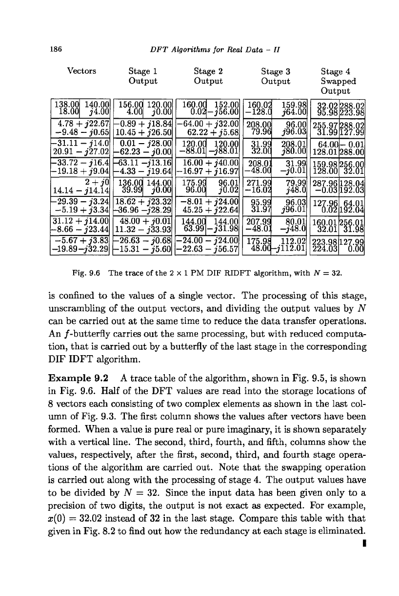
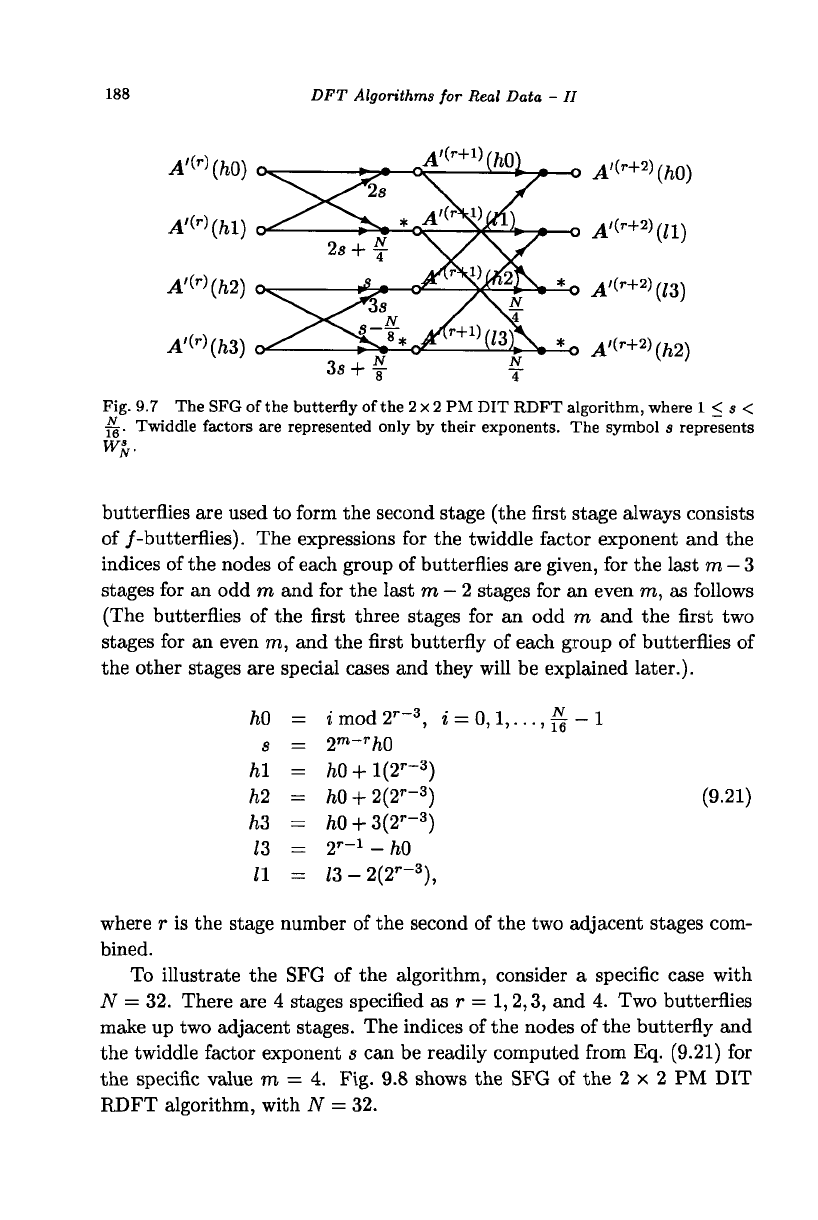
These equations characterize

the

input-output relation

the 2 x 2 PM DIT

RDFT butterfly, shown

Fig.

9.7.

The computational stages

There are

stages specified

as r = 1,2,...,

m, where

m =

log

Starting

from

the

output side, pairs

adjacent stages

are

formed using

^2x2

DIT

RDFT butterflies.

If m is

even,

f 2 x 1 PM DIT

RDFT

188

DFT Algorithms for Real Data - II

V(l3)

A'(

r+2

\h2)

Fig. 9.7 The SFG of the butterfly of the

PM DIT RDFT algorithm, where 1 < s <

j^.

Twiddle factors are represented only by their exponents. The symbol s represents

W*.

butterflies are used to form the second stage (the first stage always consists

of /-butterflies). The expressions for the twiddle factor exponent and the

indices of the nodes of each group of butterflies are given, for the last m

—

stages for an odd m and for the last m

—

2 stages for an even m, as follows

(The butterflies of the first three stages for an odd m and the first two

stages for an even m, and the first butterfly of each group of butterflies of

the other stages are special cases and they will be explained later.).

ftO

imod2

0,1,...,^

hQ+l(2

)

+ 2(2

)

+ 3(2

)

2'-

- 2(2

(9.21)

where r is the stage number of the second of the two adjacent stages com-

bined.

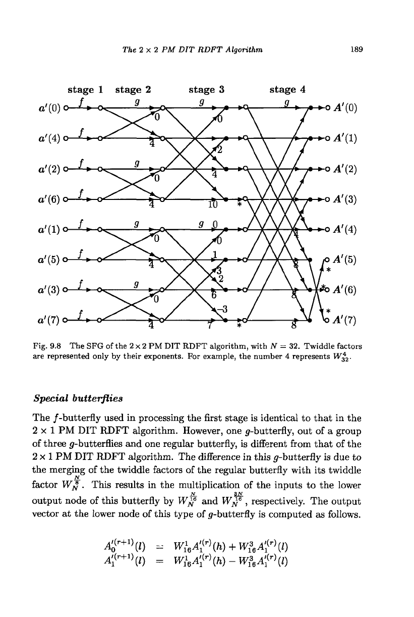
To illustrate the SFG of the algorithm, consider a specific case with

N = 32. There are 4 stages specified as r = 1,2,3, and 4. Two butterflies

make up two adjacent stages. The indices of the nodes of the butterfly and

the twiddle factor exponent s can be readily computed from Eq. (9.21) for

the specific value m = 4. Fig. 9.8 shows the SFG of the 2 x 2 PM DIT

RDFT algorithm, with N = 32.

The 2x2 PM DIT RDFT Algorithm 189

stage 1 stage 2

o'(0) o

a'(4)o

a'(2) o-^>

a'(6) o--U

a'(l)o •* » o

a'(5)c

o'(3)o

a'(7)o

stage 4

g > * *oA'(0)

•-oA'(l)

Fig. 9.8 The SFG of the 2 x 2 PM DIT RDFT algorithm, with N = 32. Twiddle factors

are represented only by their exponents. For example, the number 4 represents W£

Special butterflies

The /-butterfly used in processing the first stage is identical to that in the

2x1 PM DIT RDFT algorithm. However, one 5-butterfly, out of a group

of three ^-butterflies and one regular butterfly, is different from that of the

2 x

PM DIT RDFT algorithm. The difference in this 5-butterfly is due to

the merging of the twiddle factors of the regular butterfly with its twiddle

factor W£ . This results in the multiplication of the inputs to the lower

output node of this butterfly by Wtf and W^

, respectively. The output

vector at the lower node of this type of ^-butterfly is computed as follows.

A'(r+1)

A'l

r+1

\l)

= Wl,A'{

\h)-W*

A^\l)

190

DFT Algorithms for Real Data - II

This special 2 X 2 PM DIT RDFT butterfly requires 12 operations of real

multiplication and 34 operations of real addition.

9.5 The 2x2 PM DIF RIDFT Algorithm

By merging the multiplication operations of the adjacent stages of the 2x1

PM DIF RIDFT algorithm, we obtain the 2 x 2 PM DIF RIDFT algorithm.

The 2x2 PM DIF RIDFT butterfly

In general, the relation governing the basic computation at the rth stage is

given as

j'(r+l)

?'(r+l)

B'^'ihO)

B'^'ihO) =

r+1

\h2) =

B'}

r+1

\h2) =

{r+1)

(ll) =

r+1

\ll) =

(r+1)

(l3) =

r+1)

(l3) =

j'(r+2)

(

J3°

(p+2)

(W))

+2)

(w)

j'(H-2)

B'^'ihO)

B'o

B'„

(hO) + (B'^(l3))*

(W))-(i#

(J3))*

(hO)-W-^(B'

\l3))*

(hO) + W~

(B'

\l3))*

(ll) + (B$

\h2))*

(U)-(itf

(/i2))*

(ll)-W-*(B?

\h2))*

(Zl) + ^^"(B;

(/i2))*

r+l)

(hO) + (B'

(r+1

\ll))*

= B'J

r+1)

(hO)-(B'

{r+1

\ll)y

-28-

V(r+1) ,

W^'B[

(r+1)

{hO)

W-

~(B[

(r+l,

(ll))

-2s D'(r+1)

(r+i

>(hl) =

W^'B'i

(ho)

(B[

(r+1,

(ll)Y

{r+2

\h2)

'(r+2)

(h2) =

W^B$

r+1)

(h2)

%(B'

{r+1)

(l3))

W^B^>(h2)

^(BT

{r+2

\h3) = W^

B'}

r+1)

(h2)-W-

-^(B'}

r+1)

(l3))*

-3s-*

{r+2

>(h3) = Wj

'B?

r+1

\h2) + W-''--*{B'

(r+1

>(l3))*,

D'(r+1),

(9.22)

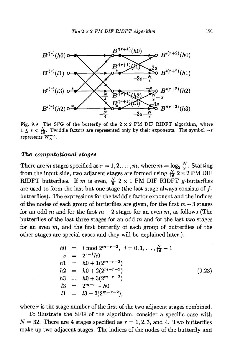
where s is an integer whose value depends on the stage of the computation

r and the index

hO.

These equations characterize the input-output relation

of the 2 x 2 PM DIF RIDFT butterfly, shown in Fig. 9.9.

The 2x2 PM DIF RIDFT Algorithm

191

B'W(ft2)o

^M_o

(/l0)

J* B'(

r+2

)(W)

B'^

)(/i2)

Fig. 9.9 The SFG of the butterfly of the 2 x 2 PM DIF RIDFT algorithm, where

1 < s < jg. Twiddle factors are represented only by their exponents. The symbol —s

represents W^

•

The computational stages

There are m stages specified as r =

1,2,...,

m, where m = log

y. Starting

from the input side, two adjacent stages are formed using ^ 2 x 2 PM DIF

RIDFT butterflies. If m is even, f 2 x 1 PM DIF RIDFT ^-butterflies

are used to form the last but one stage (the last stage always consists of f-

butterflies). The expressions for the twiddle factor exponent and the indices

of the nodes of each group of butterflies are given, for the first m

—

3 stages

for an odd m and for the first m

—

2 stages for an even m, as follows (The

butterflies of the last three stages for an odd m and for the last two stages

for an even m, and the first butterfly of each group of butterflies of the

other stages are special cases and they will be explained later.).

= 01 2- - 1

ftO

= i mod

r-2

= 2

= M + l(2

)

= h0 + 2(2

)

+ 3(2

)

= 2

= 13- 2(2

-'-

(9.23)

where r is the stage number of the first of the two adjacent stages combined.

To illustrate the SFG of the algorithm, consider a specific case with

N = 32. There are 4 stages specified as r = 1,2,3, and 4. Two butterflies

make up two adjacent stages. The indices of the nodes of the butterfly and

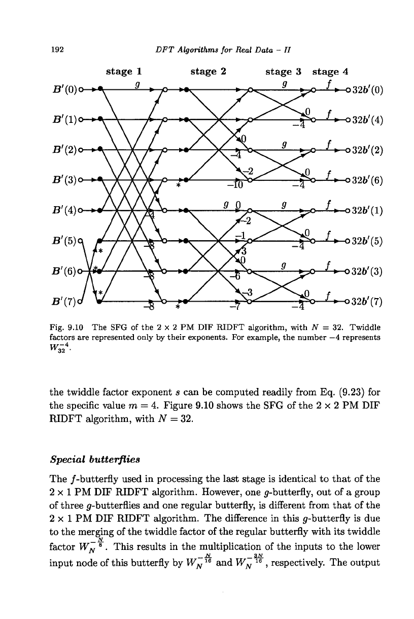
192 DFT Algorithms for Real Data - //

stage 1 stage 2 stage 3 stage 4

Fig. 9.10 The SFG of the 2 x 2 PM DIF RIDFT algorithm, with JV = 32. Twiddle

factors are represented only by their exponents. For example, the number

—4

represents

the twiddle factor exponent s can be computed readily from Eq. (9.23) for

the specific value m = 4. Figure 9.10 shows the SFG of the 2 x 2 PM DIF

RIDFT algorithm, with JV = 32.

Special butterflies

The /-butterfly used in processing the last stage is identical to that of the

2x1 PM DIF RIDFT algorithm. However, one ^-butterfly, out of a group

of three (/-butterflies and one regular butterfly, is different from that of the

2 x 1 PM DIF RIDFT algorithm. The difference in this (/-butterfly is due

to the merging of the twiddle factor of the regular butterfly with its twiddle

factor W

. This results in the multiplication of the inputs to the lower

— M. 31V

input node of this butterfly by W

and W

, respectively. The output

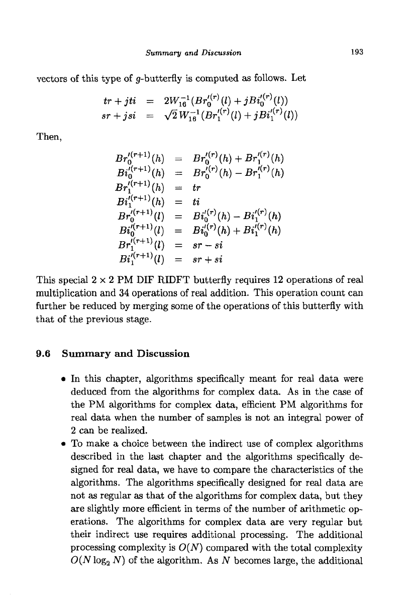
Summary

and

Discussion

193

vectors

this type

y-butterfly

computed

follows.

Let

jti =

2Wr

{B4

(l)+jB4

\l))

sr+jsi

>/2Wtf(Br;

(r)

(/)+j£»i

(r)

(0)

Then,

Br't

+l)

(h)

Bi'^W

Br[

ir+1)

{h)

Bi[

{r+1

\h)

Br'f

\l)

r+1)

Br[

ir+1

\l)

Bi'{

r+1

\l)

Br$

{h)

Br'f

\h)

Br$

{h)-Br't

(h)

Bif\h)-Bi'l

\h)

Bi'(

(h)

Bi'}

\h)

—

sr +

This special

2x2 PM

DIF

RIDFT butterfly requires

operations

real

multiplication

and 34

operations

real addition. This operation count

can

further

reduced

merging some

the operations

this butterfly with

that

the

previous stage.

9.6 Summary

and

Discussion

•

this chapter, algorithms specifically meant

for

real data were

deduced from

the

algorithms

for

complex data.

As in the

case

the

algorithms

for

complex data, efficient

algorithms

for

real data when

the

number

samples

is not an

integral power

can be

realized.

•

make

choice between

the

indirect

use of

complex algorithms

described

in the

last chapter

and the

algorithms specifically

de-

signed

for

real data,

have

compare

the

characteristics

the

algorithms.

The

algorithms specifically designed

for

real data

are

not

regular

that

the algorithms

for

complex data,

but

they

are slightly more efficient

terms

the

number

arithmetic

op-

erations.

The

algorithms

for

complex data

are

very regular

but

their indirect

use

requires additional processing.

The

additional

processing complexity

0(N)

compared with

the

total complexity

0(N log

N) of

the

algorithm.

becomes large,

the

additional