Stone M., Goldbart P. Mathematics for Physics: A Guided Tour for Graduate Students
Подождите немного. Документ загружается.

8.1 Curvilinear coordinates 265
P
y
x
r
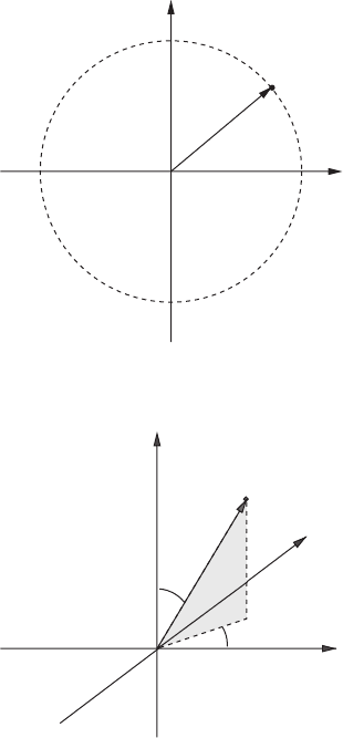
Figure 8.1 Plane polar coordinates.
x
y
z
P
r
Figure 8.2 Spherical coordinates.
Plane polar coordinates
Plane polar coordinates (Figure 8.1) have metric
ds
2
= dr
2
+ r
2
dθ
2
, (8.2)
so h
r
= 1, h
θ
= r.
Spherical polar coordinates
This system (Figure 8.2) has metric
ds
2
= dr
2
+ r
2
dθ
2
+ r
2
sin
2
θdφ
2
, (8.3)
so h
r
= 1, h
θ
= r, h
φ
= r sin θ .
266 8 Special functions
x
y
z
P
r
z
Figure 8.3 Cylindrical coordinates.
e
r
e
Figure 8.4 Unit basis vectors in plane polar coordinates.
Cylindrical polar coordinates
These have metric (Figure 8.3)
ds
2
= dr
2
+ r
2
dθ
2
+ dz
2
, (8.4)
so h
r
= 1, h
θ
= r, h
z
= 1.
8.1.1 Div, grad and curl in curvilinear coordinates
It is very useful to know how to write the curvilinear coordinate expressions for the
common operations of the vector calculus. Knowing these, we can then write down the
expression for the Laplace operator.
The gradient operator
We begin with the gradient operator. This is a vector quantity, and to express it we need
to understand how to associate a set of basis vectors with our coordinate system. The
simplest thing to do is to take unit vectors e
i
tangential to the local coordinate axes
(Figure 8.4). Because the coordinate system is orthogonal, these unit vectors will then
constitute an orthonormal system.

8.1 Curvilinear coordinates 267
The vector corresponding to an infinitesimal coordinate displacement dx
i
is then given by
dr = h
1
dx
1
e
1
+ h
2
dx
2
e
2
+ h
3
dx
3
e
3
. (8.5)
Using the orthonormality of the basis vectors, we find that
ds
2
≡|dr|
2
= h
2
1
(dx
1
)
2
+ h
2
2
(dx
2
)
2
+ h
2
3
(dx
3
)
2
, (8.6)
as before.
In the unit-vector basis, the gradient vector is
grad φ ≡∇φ =
1
h
1
∂φ
∂x
1
e
1
+
1
h
2
∂φ
∂x
2
e
2
+
1
h
3
∂φ
∂x
3
e
3
, (8.7)
so that
(grad φ) · dr =
∂φ
∂x
1
dx
1
+
∂φ
∂x
2
dx
2
+
∂φ
∂x
3
dx
3
, (8.8)
which is the change in the value φ due to the displacement.
The numbers (h
1
dx
1
, h
2
dx
2
, h
3
dx
3
) are often called the physical components of the
displacement dr, to distinguish them from the numbers (dx
1
, dx
2
, dx
3
) which are the
coordinate components of dr. The physical components of a displacement vector all have
the dimensions of length. The coordinate components may have different dimensions
and units for each component. In plane polar coordinates, for example, the units will
be meters and radians. This distinction extends to the gradient itself: the coordinate
components of an electric field expressed in polar coordinates will have units of volts
per metre and volts per radian for the radial and angular components, respectively. The
factor 1/h
θ
= r
−1
serves to convert the latter to volts per metre.
The divergence
The divergence of a vector field A is defined to be the flux of A out of an infinitesimal
region, divided by volume of the region.
In Figure 8.5, the flux out of the two end faces is
dx
2
dx
3
A
1
h
2
h
3
|
(x
1
+dx
1
,x
2
,x
3
)
− A
1
h
2
h
3
|
(x
1
,x
2
,x
3
)
≈ dx
1
dx
2
dx
3
∂(A
1
h
2
h
3
)
∂x
1
. (8.9)
Adding the contributions from the other two pairs of faces, and dividing by the volume,
h
2
h
2
h
3
dx
1
dx
2
dx
3
, gives
div A =
1
h
1
h
2
h
3
∂
∂x
1
(h
2
h
3
A
1
) +
∂
∂x
2
(h
1
h
3
A
2
) +
∂
∂x
3
(h
1
h
2
A
3
)
. (8.10)
Note that in curvilinear coordinates div A is no longer simply ∇·A, although one often
writes it as such.
268 8 Special functions
h
1
dx
1
h
2
dx
2
h
3
dx
3
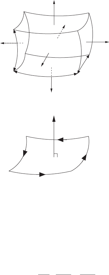
Figure 8.5 Flux out of an infinitesimal volume with sides of length h
1
dx
1
, h
2
dx
2
, h
3
dx
3
.
h
2
dx
2
h
1
dx
1
e
3
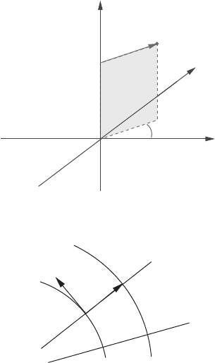
Figure 8.6 Line integral round an infinitesimal area with sides of length h
1
dx
1
, h
2
dx
2
and
normal e
3
.
The curl
The curl of a vector field A is a vector whose component in the direction of the normal
to an infinitesimal area element is the line integral of A round the infinitesimal area,
divided by the area (Figure 8.6).
The third component is, for example,
(curl A)
3
=
1
h
1
h
2
∂h
2
A
2
∂x
1
−
∂h
1
A
1
∂x
2
. (8.11)
The other two components are found by cyclically permuting 1 → 2 → 3 → 1 in this
formula. The curl is thus is no longer equal to ∇×A, although it is common to write it
as if it were.
Note that the factors of h
i
are disposed so that the vector identities
curl grad ϕ = 0, (8.12)

8.1 Curvilinear coordinates 269
and
div curl A = 0, (8.13)
continue to hold for any scalar field ϕ, and any vector field A.
8.1.2 The Laplacian in curvilinear coordinates
The Laplacian acting on scalars is “div grad”, and is therefore
∇
2
ϕ =
1
h
1
h
2
h
3
∂
∂x
1
h
2
h
3
h
1
∂ϕ
∂x
1
+
∂
∂x
2
h
1
h
3
h
2
∂ϕ
∂x
2
+
∂
∂x
3
h
1
h
2
h
3
∂ϕ
∂x
3
. (8.14)
This formula is worth committing to memory.
When the Laplacian is to act on a vector field, we must use the vector Laplacian
∇
2
A = grad div A −curl curl A. (8.15)
In curvilinear coordinates this is no longer equivalent to the Laplacian acting on each
component of A, treating it as if it were a scalar. The expression (8.15) is the appropriate
generalization of the vector Laplacian to curvilinear coordinates because it is defined
in terms of the coordinate independent operators div, grad and curl, and reduces to the
Laplacian on the individual components when the coordinate system is cartesian.
In spherical polars the Laplace operator acting on the scalar field ϕ is
∇
2
ϕ =
1
r
2
∂
∂r
r
2
∂ϕ
∂r
+
1
r
2
sin θ
∂
∂θ
sin θ
∂ϕ
∂θ
+
1
r
2
sin
2
θ
∂
2
ϕ
∂φ
2
=
1
r
∂
2
(rϕ)
∂r
2
+
1
r
2
1
sin θ
∂
∂θ
sin θ
∂ϕ
∂θ
+
1
sin
2
θ
∂
2
ϕ
∂φ
2
=
1
r
∂
2
(rϕ)
∂r
2
−
ˆ
L
2
r
2
ϕ, (8.16)
where
ˆ
L
2
=−
1
sin θ
∂
∂θ
sin θ
∂
∂θ
−
1
sin
2
θ
∂
2
∂φ
2
, (8.17)
is (after multiplication by
2
) the operator representing the square of the angular
momentum in quantum mechanics.
In cylindrical polars the Laplacian is
∇
2
=
1
r
∂
∂r
r
∂
∂r
+
1
r
2
∂
2
∂θ
2
+
∂
2
∂z
2
. (8.18)

270 8 Special functions
8.2 Spherical harmonics
We saw that Laplace’s equation in spherical polars is
0 =
1
r
∂
2
(rϕ)
∂r
2
−
ˆ
L
2
r
2
ϕ. (8.19)
To solve this by the method of separation of variables, we factorize
ϕ = R(r)Y (θ , φ), (8.20)
so that
1
Rr
d
2
(rR)
dr
2
−
1
r
2
1
Y
ˆ
L
2
Y
= 0. (8.21)
Taking the separation constant to be l(l + 1), we have
r
d
2
(rR)
dr
2
− l(l + 1)(rR) = 0, (8.22)
and
ˆ
L
2
Y = l(l + 1)Y . (8.23)
The solution for R is r
l
or r
−l−1
. The equation for Y can be further decomposed by
setting Y = !(θ)(φ). Looking back at the definition of
ˆ
L
2
, we see that we can take
(φ) = e
imφ
(8.24)
with m an integer to ensure single-valuedness. The equation for ! is then
1
sin θ
d
dθ
sin θ
d!
dθ
−
m
2
sin
2
θ
! =−l(l + 1)!. (8.25)
It is convenient to set x = cos θ; then
d
dx
(1 − x
2
)
d
dx
+ l(l + 1) −
m
2
1 − x
2
! = 0. (8.26)
8.2.1 Legendre polynomials
We first look at the axially symmetric case where m = 0. We are left with
d
dx
(1 − x
2
)
d
dx
+ l(l + 1)
! = 0. (8.27)

8.2 Spherical harmonics 271
This is Legendre’s equation. We can think of it as an eigenvalue problem
−
d
dx
(1 − x
2
)
d
dx
!(x) = l(l + 1)!(x), (8.28)
on the interval −1 ≤ x ≤ 1, this being the range of cos θ for real θ . Legendre’s
equation is of Sturm–Liouville form, but with regular singular points at x =±1. Because
the endpoints of the interval are singular, we cannot impose as boundary conditions
that !, !
, or some linear combination of these, be zero there. We do need some
boundary conditions, however, so as to have a self-adjoint operator and a complete set
of eigenfunctions.
Given one or more singular endpoints, a possible route to a well-defined eigenvalue
problem is to require solutions to be square-integrable, and so normalizable. This condi-
tion suffices for the harmonic-oscillator Schrödinger equation, for example, because at
most one of the two solutions is square-integrable. For Legendre’s equation with l = 0,
the two independent solutions are !(x) = 1 and !(x) = ln(1 + x) − ln(1 − x). Both
of these solutions have finite L
2
[−1, 1] norms, and this square integrability persists for
all values of l. Thus, demanding normalizability is not enough to select a unique bound-
ary condition. Instead, each endpoint possesses a one-parameter family of boundary
conditions that lead to self-adjoint operators. We therefore make the more restrictive
demand that the allowed eigenfunctions be finite at the endpoints. Because the north and
south poles of the sphere are not special points, this is a physically reasonable condition.
When l is an integer, then one of the solutions, P
l
(x), becomes a polynomial, and so is
finite at x =±1. The second solution Q
l
(x) is divergent at both ends, and so is not an
allowed solution. When l is not an integer, neither solution is finite. The eigenvalues
are therefore l(l + 1) with l zero or a positive integer. Despite its unfamiliar form, the
“finite” boundary condition makes the Legendre operator self-adjoint, and the Legendre
polynomials P
l
(x) form a complete orthogonal set for L
2
[−1, 1].
Proving orthogonality is easy: we follow the usual strategy for Sturm–Liouville
equations with non-singular boundary conditions to deduce that
[l(l + 1) − m(m + 1)]
1
−1
P
l
(x)P
m
(x) dx =
7
(P
l
P
m
− P
l
P
m
)(1 − x
2
)
8
1
−1
. (8.29)
Since the P
l
’s remain finite at ±1, the right-hand side is zero because of the (1 − x
2
)
factor, and so
1
−1
P
l
(x)P
m
(x) dx is zero if l = m. (Observe that this last step differs from
the usual argument where it is the vanishing of the eigenfunction or its derivative that
makes the integrated-out term zero.)
Because they are orthogonal polynomials, the P
l
(x) can be obtained by applying the
Gram–Schmidt procedure to the sequence 1, x, x
2
, ...to obtain polynomials orthogonal
with respect to the w ≡ 1 inner product, and then fixing the normalization constant. The
result of this process can be expressed in closed form as
P
l
(x) =
1
2
l
l!
d
l
dx
l
(x
2
− 1)
l
. (8.30)

272 8 Special functions
This is called Rodriguez’formula. It should be clear that this formula outputs a polynomial
of degree l. The coefficient 1/2
l
l! comes from the traditional normalization for the
Legendre polynomials that makes P
l
(1) = 1. This convention does not lead to an
orthonormal set. Instead, we have
1
−1
P
l
(x)P
m
(x) dx =
2
2l + 1
δ
lm
. (8.31)
It is easy to show that this integral is zero if l > m – simply integrate by parts l times
so as to take the l derivatives off (x
2
−1)
l
and onto (x
2
−1)
m
, which they kill. We will
evaluate the l = m integral in the next section.
We now show that the P
l
(x) given by Rodriguez’ formula are indeed solutions of
Legendre’s equation: let v = (x
2
− 1)
l
, then
(1 − x
2
)v
+ 2lxv = 0. (8.32)
We differentiate this l + 1 times using Leibniz’ theorem
[uv]
(n)
=
n
m=0
n
m
u
(m)
v
(n−m)
= uv
(n)
+ nu
v
(n−1)
+
1
2
n(n − 1)u
v
(n−2)
+ .... (8.33)
We find that
[(1 − x
2
)v
]
(l+1)
= (1 − x
2
)v
(l+2)
− (l +1)2xv
(l+1)
− l(l + 1)v
(l)
,
[2xnv]
(l+1)
= 2xlv
(l+1)
+ 2l(l + 1)v
(l)
. (8.34)
Putting these two terms together we obtain
(1 − x
2
)
d
2
dx
2
− 2x
d
dx
+ l(l + 1)
d
l
dx
l
(x
2
− 1)
l
= 0, (8.35)
which is Legendre’s equation.
The P
l
(x) have alternating parity
P
l
(−x) = (−1)
l
P
l
(x), (8.36)
and the first few are
P
0
(x) = 1,
P
1
(x) = x,
8.2 Spherical harmonics 273
P
2
(x) =
1
2
(3x
2
− 1),
P
3
(x) =
1
2
(5x
3
− 3x),
P
4
(x) =
1
8
(35x
4
− 30x
2
+ 3).
8.2.2 Axisymmetric potential problems
The essential property of the P
l
(x) is that the general axisymmetric solution of ∇
2
ϕ = 0
can be expanded in terms of them as
ϕ(r, θ) =
∞
l=0
A
l
r
l
+ B
l
r
−l−1
P
l
(cos θ). (8.37)
You should memorize this formula. You should also know by heart the explicit expres-
sions for the first four P
l
(x), and the factor of 2/(2l + 1) in the orthogonality
formula.
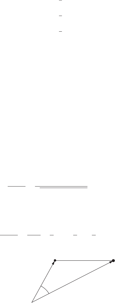
Example: Point charge. Put a unit charge at the point R, and find an expansion for the
potential as a Legendre polynomial series in a neighbourhood of the origin (Figure 8.7).
Let us start by assuming that |r| < |R|. We know that in this region the point charge
potential 1/|r − R| is a solution of Laplace’s equation, and so we can expand
1
|r − R|
≡
1
√
r
2
+ R
2
− 2rR cos θ
=
∞
l=0
A
l
r
l
P
l
(cos θ). (8.38)
We knew that the coefficients B
l
were zero because ϕ is finite when r = 0. We can find
the coefficients A
l
by setting θ = 0 and Taylor expanding
1
|r − R|
=
1
R − r
=
1
R
1 +
r
R
+
r
R
2
+···
, r < R. (8.39)
R
r
| R r|
O
Figure 8.7 Geometry for generating function.

274 8 Special functions
By comparing the two series and noting that P
l
(1) = 1, we find that A
l
= R
−l−1
. Thus
1
√
r
2
+ R
2
− 2rR cos θ
=
1
R
∞
l=0
r
R
l
P
l
(cos θ), r < R. (8.40)
This last expression is the generating function formula for Legendre polynomials. It is
also a useful formula to have in your long-term memory.
If |r| > |R|, then we must take
1
|r − R|
≡
1
√
r
2
+ R
2
− 2rR cos θ
=
∞
l=0
B
l
r
−l−1
P
l
(cos θ), (8.41)
because we know that ϕ tends to zero when r =∞. We now set θ = 0 and compare with
1
|r − R|
=
1
r − R
=
1
r
1 +
R
r
+
R
r
2
+···
, R < r, (8.42)
to get
1
√
r
2
+ R
2
− 2rR cos θ
=
1
r
∞
l=0
R
r
l
P
l
(cos θ), R < r. (8.43)
Observe that we made no use of the normalization integral
1
−1
{P
l
(x)}
2
dx = 2/(2l + 1) (8.44)
in deriving the generating function expansion for the Legendre polynomials. The follow-
ing exercise shows that this expansion, taken together with their previously established
orthogonality property, can be used to establish (8.44).
Exercise 8.1: Use the generating function for Legendre polynomials P
l
(x) to show that
∞
l=0
z
2l
1
−1
{P
l
(x)}
2
dx
=
1
−1
1
1 − 2xz + z
2
dx =−
1
z
ln
1 − z
1 + z
, |z| < 1.
By Taylor expanding the logarithm, and comparing the coefficients of z
2l
, evaluate
1
−1
{P
l
(x)}
2
dx.
Example: A planet is spinning on its axis and so its shape deviates slightly from a perfect
sphere (Figure 8.8). The position of its surface is given by
R(θ, φ) = R
0
+ ηP
2
(cos θ). (8.45)