Stewart J. College Algebra: Concepts and Contexts

214 CHAPTER 2

■

Linear Functions and Models

Set y-values equal

Subtract 5t, add 2400

Divide by 3

So the cyclists meet when Jordanna has cycled for 800 seconds, or

minutes. Since Petra left 5 minutes later, she travels

minutes to catch up with Jordanna.

To find how far the cyclists have traveled when they meet, we replace t by

800 in either one of the equations.

Replace t by 800 in Jordanna’s equation

So they have cycled 4000 meters when they meet.

■ NOW TRY EXERCISE 33 ■

y = 518002= 4000

13.3 - 5 = 8.3

800>60 L 13.3

t = 800

3 t = 2400

8 t - 2400 = 5t

■ Modeling Supply and Demand

Economists model supply and demand for a commodity using linear functions. For

example, for a certain commodity we might have

where p is the price of the commodity. In the supply equation, y (the amount produced)

increases as the price increases because if the price is high, more suppliers will manu-

facture the commodity. The demand equation indicates that y (the amount sold)de-

creases as the price increases. The equilibrium point is the point of intersection of the

graphs of the supply and demand equations; at that point, the amount produced equals

the amount sold.

Demand equation:

y =-3p + 15

Supply equation: y = 8p - 10

example

Supply and Demand for Wheat

An economist models the market for wheat by the following equations.

Here, p is the price per bushel (in dollars), and y is the number of bushels produced

and sold (in millions).

(a) Use the model for supply to determine at what point the price is so low that no

wheat is produced.

(b) Use the model for demand to determine at what point the price is so high that

no wheat is sold.

Solution

(a) If no wheat is produced, then y  0 in the supply equation.

Set y  0 in the supply equation

Solve for p

p L 2.75

0 = 3.82p - 10.51

Demand:y =-0.99p + 25.34

Supply:y = 3.82p - 10.51

SECTION 2.7

■

Linear Equations: Where Lines Meet 215

So at the low price of $2.75 per bushel, the production of the wheat halts

completely.

(b) If no wheat is sold, then in the demand equation.

Set y  0 in the demand equation

Solve for p

So at the high price of $25.60 per bushel, no wheat is sold.

to each other and solve.

Set functions equal

Add 10.51

Add 0.99p

Divide by 4.81

So the equilibrium price is $7.45. Evaluating the supply equation for ,

we get

So for the equilibrium price of $7.45 per bushel, about 18 million bushels of

wheat are produced and sold.

■ NOW TRY EXERCISE 35 ■

y = 3.8217.452- 10.51 L 17.95

p = 7.45

p L 7.45

4.81p = 35.85

3.82p =-0.99p + 35.85

3.82p - 10.51 =-0.99p + 25.34

p L 25.60

0 =-0.99p + 25.34

y = 0

2.7 Exercises

Fundamentals

1. (a) To find where the graphs of the functions and

intersect, we solve for x in the equation

_______ _______

(b) To find where the graphs of the functions and intersect,

we solve for x in the equation

_______ _______. So the graphs of these

functions intersect when x 

_______. Therefore the graphs intersect at the point

(____, ____).

2. (a) The point where the graphs of supply and demand equations intersect is called the

______________ point.

(b) The supply of a product is given by the equation , and the demand is

given by the equation , where p is the price of the product. To find

the price for which supply is equal to demand, we solve for p in the equation

______________  ______________.

Think About It

3. Muna’s and Michael’s distances from home are modeled by the following equations.

Explain why Michael will never catch up with Muna.

Michael’s equation:

y = 2 + 3t

Muna’s equation:

y = 4 + 3t

y = m

p + b

y = m

p + b

y = 3x - 10y = 2x + 7

y = m

x + b

y = m

x + b

CONCEPTS

216 CHAPTER 2

■

Linear Functions and Models

SKILLS

1_1 2345

4. Udit is walking from school to his home 5 miles away, starting at time t  0. Udit walks

slowly at a speed of 2 miles per hour. If the time t is measured in hours, then

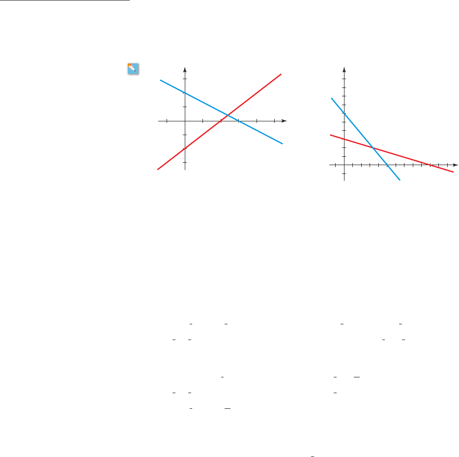
5–6 ■ A graph of two lines is given.

(a) Use the graph to estimate the coordinates of the point of intersection.

(b) Find an equation for each line.

Compare with your answer to part (a).

5. 6.

Udit’s distance from home at time t is y =

ⵧ

Udit’s distance from school at time t is y =

ⵧ

7–10

■ Linear functions f and are given.

(a) Graph f and , and use the graphs to estimate the value of x where the graphs

intersect.

(b) Find algebraically the value of x where the graphs of f and intersect.

7. ; 8. ;

9. ; 10. ;

11–16

■ Find the value of x for which the graphs of the two linear equations intersect.

11. ; y  x 12. ; y  7  x

13. ; 14. ;

15. ; 16. ;

17–22

■ Find the point at which the graphs of the two linear equations intersect.

17. ; 18. ;

19. ; 20. ;

21. ; 22. ;

23–24

■ Two linear functions are described verbally. Find equations for the functions, and

find the point at which the graphs of the two functions intersect.

23. The graph of the linear function f has slope and y-intercept 5; the graph of the linear

function has slope 5 and y-intercept 2.

24. The graph of the linear function f has x-intercept 4 and y-intercept ; the graph of the

linear function has x-intercept and y-intercept 10.

25–26

■ Equations for supply and demand are given. Find the price (in dollars) and the

amount of the commodity produced and sold at equilibrium.

- 2g

- 1

y = 6.6 + 0.6xy = 9 + xy =

x - 12y = 6 -

y = 40 - 3xy =

xy = 5x - 2y =

y = 9x + 6y =

x -

y =

x + 3y = 2 + x

y =

x +

y = 7 - xy = 2x - 3y =

y =-4 -

xy =-

xy =

x - 3y = 3 -

y  x  3y = 4 - x

g1x 2=-3x + 6f 1x 2= 2x - 4g1x 2=-2x + 2f 1x2= x - 4

g1x 2=-x - 1f 1x2= x + 3g1x 2=-2x + 3f 1x 2= 2x - 5

SECTION 2.7

■

Linear Equations: Where Lines Meet 217

25. 26.

27. Cell Phone Plan Comparison Dietmar is in the process of choosing a cell phone and

a cell phone plan. The first plan charges 20¢ per minute plus a monthly fee of $10, and

the second plan offers unlimited minutes for a monthly fee of $100.

(a) Find a linear function f that models the monthly cost of the first plan in terms

of the number x of minutes used.

(b) Find a linear function that models the monthly cost of the second plan in

terms of the number x of minutes used.

monthly cost.

28. Solar Power Lina is considering installing solar panels on her house. Solar

Advantage offers to install solar panels that generate 320 kWh of electricity per month

for an installation fee of $15,000. She uses 350 kWh of electricity per month, and her

local utility company charges 20¢ per kWh.

(a) If Lina gets all her electrical power from the local utility company, find a linear

function U that models the cost of electricity for x months of service.

(b) If Lina has Solar Advantage install solar panels on her roof that generate 320 kWh

of power per month, find a linear function S that models the cost S(x) of electricity

for x months of service.

for installation of Solar Advantage’s solar panels, that is, determine when .

29. Renting Versus Buying a Photocopier A certain office can purchase a photocopier

for $5800 with a maintenance fee of $25 a month. On the other hand, they can rent the

photocopier for $95 a month (including maintenance). If they purchase the photocopier,

each copy would cost 3¢; if they rent, the cost is 6¢ per copy. The office manager

estimates that they make 8000 copies a month.

(a) Find a linear function C that models the cost of purchasing and using the

copier for x months.

(b) Find a linear function S that models the cost of renting and using the copier

for x months.

increments.

(d) For how many months of use would the cost be the same for each method?

30. Cost and Revenue A tire company determines that to manufacture a certain type of

tire, it costs $8000 to set up the production process. Each tire that is produced costs $22

in material and labor. The company sells this tire to wholesale distributors for $49 each.

(a) Find a linear function C that models the total cost of producing x tires.

(b) Find a linear function R that models the revenue from selling x tires.

[Note: .]

(d) How many tires must the company sell to break even (that is, when does revenue

equal cost)?

31. Car Rental A businessman intends to rent a car for a 3-day business trip. The rental is

$35 a day and 15¢ per mile (Plan 1) or $90 a day with unlimited mileage (Plan 2). He is not

sure how many miles he will drive but estimates that it will be between 1000 and 1200 miles.

(a) For each plan, find a linear function

C that models the cost in terms of the

number x of miles driven.

(b) Which rental plan is cheaper if the businessman drives 1000 miles? 1200 miles? At

what mileage do the two plans cost the same?

C 1x 2

profit = revenue - cost

P 1x 2

R 1x 2

C 1x 2

S 1x 2

C 1x 2

S 1x 2= U 1x2

U 1x 2

g1x 2g

f 1x 2

Demand: y =-0.6p + 300Demand: y =-0.65p + 28

Supply: y = 8.5p + 45Supply: y = 0.45p + 4

CONTEXTS

218 CHAPTER 2

■

Linear Functions and Models

32. Buying a Car Kofi wants to buy a new car, and he has narrowed his choices to two

models.

Model A sells for $15,500, gets 25 mi/gal, and costs $350 a year for insurance

Model B sells for $19,100, gets 48 mi/gal, and costs $425 a year for insurance

Kofi drives about 36,000 miles a year, and gas costs about $4.50 a gallon.

(a) Find a linear function A that models the total cost of owning Model A for

x years.

(b) Find a linear function B that models the total cost of owning Model B for

x years.

A equals the cost of owning Model B.

33. Commute to Work (See Exercise 59 in Section 2.2.) Jade and her roommate Jari live

in a suburb of San Antonio, Texas, and both work at an elementary school in the city.

Each morning they commute to work traveling west on I-10. One morning Jade leaves

for work at 6:50

A.M., but Jari leaves 10 minutes later. On this trip Jade drives at an

average speed of 65 mi/h, and Jari drives at an average speed of 72 mi/h.

(a) Find a linear equation that models the distance y Jari has traveled x hours after she

leaves home.

(b) Find a linear equation that models the distance y Jade has traveled x hours after Jari

leaves home.

at the time they meet?

34. Catching Up Kumar leaves his house at 7:30

A.M. and cycles to school. Kumar’s

mother notices that he has left his lunch at home. She leaves the house by car 5 minutes

after Kumar left to give him his lunch. Kumar cycles at an average speed of 8 mi/h, and

his mother drives at an average speed of 24 mi/h.

(a) Find a linear equation that models the distance y Kumar’s mother has traveled x

hours after she left home.

(b) Find a linear equation that models the distance y Kumar has traveled x hours after

his mother has left home.

(d) Determine how long it takes Kumar’s mother to catch up with Kumar. How far have

they traveled at the time they meet?

35. Supply and Demand for Corn An economist models the market for corn by the

following equations:

Here, p is the price per bushel (in dollars), and y is the number of bushels produced and

sold (in billions).

(a) Use the model for supply to determine at what point the price is so low that no corn

is produced.

(b) Use the model for demand to determine at what point the price is so high that no

corn is sold.

equilibrium.

36. Supply and Demand for Soybeans An economist models the market for soybeans

by the following equations:

Demand:

y =-0.23p + 5.22

Supply:

y = 0.37p - 1.59

Demand:

y =-1.06p + 19.3

Supply:

y = 4.18p - 11.5

B 1x 2

A 1x 2

CHAPTER 2

■

Review 219

Here p is the price per bushel (in dollars), and y is the number of bushels produced and

sold (in billions).

(a) Use the model for supply to determine at what point the price is so low that no

soybeans are produced.

(b) Use the model for demand to determine at what point the price is so high that no

soybeans are sold.

equilibrium.

37. Median Incomes of Men and Women The gap between the median income of men

and that of women has been slowly shrinking over the past 30 years. Search the Internet

to find the median incomes of men and women for 1965 to 2005.

(a) Find the regression line for the data found on the Internet for the median income

of men.

(b) Find the regression line for the data found on the Internet for the median income

of women.

median incomes of men and women will be the same.

38. Population The populations in many large metropolitan districts have recently been

decreasing as residents move to the suburbs. Search the Internet for a city of your

choice where there has been a decrease in the metropolitan population and an increase

in the suburban population.

(a) Find the regression line for the metropolitan population data for the past 40 years.

(b) Find the regression line for the suburban population data for the past 40 years.

suburban population will equal the metropolitan population.

39. Teacher Salaries The gap between the median salaries for men teachers and women

teachers has recently been shrinking. Search the Internet to find a history for the past

30 years of men and women teachers’ median salaries in your state.

(a) Find the regression line for the data on the men teachers’ median salary.

(b) Find the regression line for the data on the women teachers’ median salary.

median teacher’s salary will be equal for men and women.

CHAPTER 2

REVIEW

CONCEPT CHECK

Make sure you understand each of the ideas and concepts that you learned in this chapter,

as detailed below section by section. If you need to review any of these ideas, reread the

appropriate section, paying special attention to the examples.

2.1 Working with Functions: Average Rate of Change

The average rate of change of the function between x  a and x  b is

average rate of change =

net change in y

change in x

f 1b 2- f 1a2

b - a

y = f 1x2

CHAPTER

220 CHAPTER 2

■

Linear Functions and Models

The average rate of change measures how quickly the dependent variable changes

with respect to the independent variable. A familiar example of a rate of change is

the average speed of a moving object such as a car.

2.2 Linear Functions: Constant Rate of Change

A linear function is a function of the form . Such a function is called

linear because its graph is a straight line. The average rate of change of a linear func-

tion between any two values of x is always m, so we refer to m simply as the rate of

change of f. The number b is the starting value of the function (its value when x is 0).

To find the slope of a line graphed in a coordinate plane, we choose two differ-

ent points on the line, and , and calculate

The y-intercept of the graph of any function f is

If is a linear function, then

■

The graph of f is a line with slope m.

■

The y-intercept of the graph of f is b.

Thus the rate of change of f is the slope of its graph, and the initial value of f is the

y-intercept of its graph.

2.3 Equations of Lines: Constructing Linear Models

A linear model is a linear function that models a real-life situation. To construct a

linear model from data or from a verbal description of the situation, we use one of

the following equivalent forms of the equation of a line:

■

Slope-intercept form:

when we know the slope m and the y-intercept b.

■

Point-slope form:

when we know the slope m and a point that lies on the line.

If we know two points that lie on a line, we first use the points to find the slope

m and then use this slope and one of the given points in the point-slope form to find

the equation of the line.

Horizontal and vertical lines have simple equations:

■

The vertical line through the point (a, b) has equation x  a.

■

The horizontal line through the point (a, b) has equation y  b.

The general form of the equation of a line is

Every line has an equation of this form, and the graph of every equation of this form

is a line.

2.4 Varying the Coefficients: Direct Proportionality

The numbers b and m in the linear equation are called the coefficients

of the equation: b is the constant coefficient and m is the coefficient of x.

If two nonvertical lines have slopes and , then they arem

y = b + mx

Ax + By + C = 0

, y

y - y

= m 1x - x

y = b + mx

f 1x2= b + mx

f 10 2.

slope 

rise

run



change in y

change in x



 y

 x

, y

21x

, y

f 1x 2= b + mx

CHAPTER 2

■

Review 221

■

parallel if they have the same slope: .

■

perpendicular if they have negative reciprocal slopes: .

The variable y is directly proportional to the variable x (or y varies directly as x)

if there is a constant k such that x and y are related by the equation y  kx. The constant

k is called the constant of proportionality. The graph of a proportionality equation is

a straight line with slope k passing through the origin.

2.5 Linear Regression: Fitting Lines to Data

In Section 2.3 we found linear models for data whose scatter plots lie exactly on a

line. Most real-life data are not exactly linear but may appear to lie approximately on

a line. In this case a linear model can still be useful for revealing trends and patterns.

The linear model that we use is called the regression line; it is the “line of best fit”

for the data.

A simple way to find the regression line for a set of data is to use a graphing cal-

culator. (The command for this is LinReg on many calculators.)

A regression line can be found for any set of two-variable data, but this line

isn’t meaningful if too many of the data points lie far away from the line in a scat-

ter plot. The correlation coefficient r is a measure of how closely data fit their re-

gression line (that is, how closely the variables correlate). For any regression line

we have ; values of r close to 1 or indicate a high degree of corre-

lation, and values of r close to 0 indicate little or no correlation.

2.6 Linear Equations: Getting Information from a Model

To construct a model from a verbal description of a real-life situation, we follow

three general steps:

1. Choose the variable in terms of which the model will be expressed. Assign a

symbol (such as x) to the variable.

2. Translate words into algebra by expressing the other quantities in the problem

in terms of the variable x.

3. Set up the model by expressing the fact(s) given about the quantity modeled as

a function of x.

Once we have found a model, we can use it to answer questions about the quantity

being modeled. This will often require solving equations.

2.7 Linear Equations: Where Lines Meet

Some models involve two linear functions that model two different but related quan-

tities. We are often interested in determining when the two functions have the same

value. In this case we need to find the point at which the graphs of the two lines meet.

This can be accomplished in one of two ways:

■

Graphically, by graphing both lines on the same coordinate plane and esti-

mating the coordinates of the point of intersection

■

Algebraically, by setting the two functions equal to each other and solving

the resulting equation

The graphical method usually gives just an estimate, but the algebraic method

always gives the exact answer.

- 1- 1 … r … 1

= -

= m

x f(x)

2 5.5

6 4.5

222 CHAPTER 2

■

Linear Functions and Models

REVIEW EXERCISES

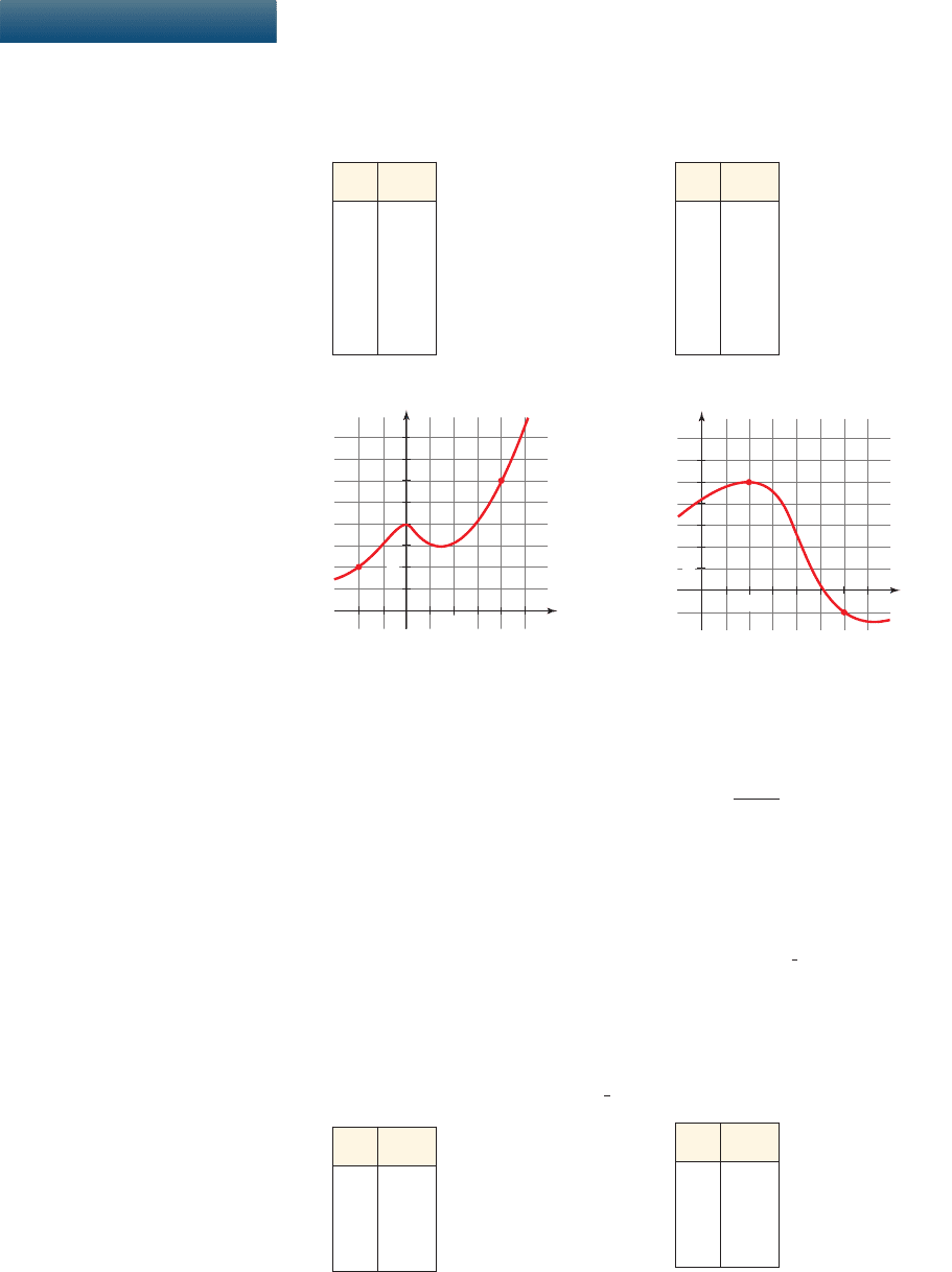
1–6 ■ A function is given (either numerically, graphically, or algebraically). Find the

average rate of change of the function between the indicated points.

1. Between x  4 and x  10 2. Between x  10 and x  30

x F(x)

412

612

10 6

12 3

x G(x)

- 5

20 10

30 30

40 0

50 15

CHAPTER

SKILLS

3. Between and x  2 4. Between x  1 and x  3x =-1

5. , between x  1 and x  4

6. , between and t  3

7–8

■ Determine whether the given function is linear.

7. 8.

9–12

■ A linear function is given.

(a) Sketch a graph of the function.

(b) What is the slope of the graph?

9. 10. 11. 12.

13–18

■ A linear function f is described, either verbally, numerically, or graphically.

Express f in the form .

13. The function has rate of change and initial value 10.

14. The graph of the function has slope and initial value 2.

15. 16.

- 5

f 1x 2= b + mx

g1x 2=-3 + xg1x 2= 3 -

xf 1x 2= 6 - 2xf 1x 2= 3 + 2x

g1x 2=

x + 5

f 1x 2= 12 + 3x2

t =-1g1t 2= 6t

- t

f 1x 2= x

+ 2x

CHAPTER 2

■

Review Exercises 223

17. 18.

27. The line is horizontal and has y-intercept 26.

28. The line is vertical and passes through the point .

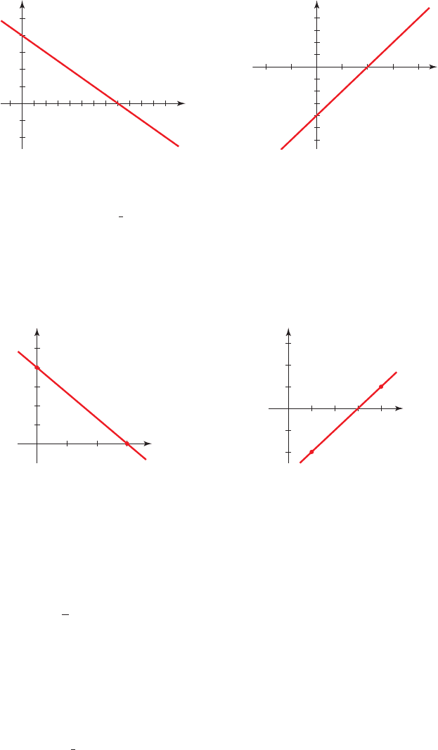
29–32

■ An equation of a line is given.

(a) Find the slope, the y-intercept, and the x-intercept of the line.

(b) Sketch a graph of the line.

29. 30.

31. 32.

33–34

■ An equation of a line l and the coordinates of a point P are given.

(a) Find an equation in general form of the line parallel to l passing through P.

(b) Find an equation in general form of the line perpendicular to l passing through P.

33. 34.

35–38

■ Find an equation for the line that satisfies the given conditions.

35. Passes through the origin, parallel to the line

36. Passes through , perpendicular to the y-axis

37. Passes through , perpendicular to the line

38. Passes through , parallel to the line that contains (1, 2) and (3, 8)1- 2, 42

x + 4y + 8 = 013, - 22

14, - 32

2x - 4y = 8

2x + 3y = 6;

P 1- 1, 22y =-2 +

x;P 12, - 32

5x + 4y + 20 = 03x - 4y - 12 = 0

3 + x = 6 + 2y1 - y =

1- 3, 262

19–28

■ Find the equation, in slope-intercept form, of the line described.

19. The line has slope 5 and y-intercept 0.

20. The line has slope and y-intercept 4.

21. The line has slope and passes through the point (1, 3).

22. The line has slope 0.25 and passes through the point .

23. The line passes through the points (2, 4) and (4, 0).

24. The line passes through the points and .

25. 26.

16, 2 21- 3, 02

1- 6, - 32

- 6

2 4 6 8 10 12

241_1_2 3

Stewart J. College Algebra: Concepts and Contexts

Подождите немного. Документ загружается.