Steve M., Darby D.M., Geostatistics Explained - An Introductory Guide for Earth Scientists

Подождите немного. Документ загружается.

may be related together in a non-linear way. The Pearson correlation

coeﬃcient is a statistic that shows the extent to which two variables are

linearly related, and can have a value between –1.0 and 1.0, with these

extremes showing a perfect negative linear relationship and perfect positive

linear relationship respectively, while zero shows no relationship. The value

of r indicates the way in which the variables are related, but the probability

of getting a particular r value is needed to decide whether the correlation is

statistically signiﬁcant.

15.8 Questions

(1) (a) Add appropriate words to the following sentence to specify a

regression analysis. “I am interested in ﬁnding out whether the shell

weight of the fossil snail Littoraria articulata...................... shell length.”

(b) Add appropriate words to the following sentence to specify a

correlation analysis. “I am interested in ﬁnding out whether the shell

weight of the fossil snail Littoraria articulata.........................shell length.”

(2) Run a correlation analysis on the following set of 10 bivariate data,

given as the values of (X,Y) for each unit: (1,5) (2,6) (3,4) (4,5) (5,5)

(6,4) (7,6) (8,5) (9,6) (10,4). (a) What is the value of the correlation

coeﬃcient? (You might draw a scatter plot of the data to help visualize

the relationship.) (b) Next, modify some of the Y values only to give a

highly signiﬁcant positive correlation between X and Y. Here a scatter

plot might help you decide how to do this. (c) Finally, modify some of

the Y values only to give a highly signiﬁcant negative correlation

between X and Y.

15.8 Questions 203

16 Linear regression

16.1 Introduction

This chapter explains simple linear regression analysis. The diﬀerent uses of

correlation and regression were contrasted in Chapter 15. Correlation

examines if two variables are related. Regression describes the functional

relationship between a dependent and an independent variable.

16.2 Linear regression

Linear regression analysis is often used by earth scientists. For example, the

equation for the regression of one variable on another may suggest hyp-

otheses about why the two variables are related. More practically, regression

can be used in situations where the dependent variable is diﬃcult, expensive

or impossible to measure, but its values can be predicted from another easily

measured variable to which it is functionally related. Here is an example.

It can be quite diﬃcult to measure the temperature of an erupting magma.

In situ measurements can be made if you can safely get close enough to lower

a sheathed thermocouple into the hot lava, but this is a dangerous under-

taking. Optical pyrometers can be used to estimate magma temperatures from

any distant position with a direct line of sight, but corrections for distance,

elevation and air temperatures must be applied.

Fortunately, it has been shown that the SiO

content of the magma varies

inversely with eruption temperature: basaltic magmas tend to erupt at

hotter temperatures (~1200–1300 °C) and more silicic ones at cooler tem-

peratures (~700–800 °C). So eruption temperature can be predicted from

the SiO

content of the cooled magma, which can be accurately (and safely)

measured in the laboratory after the eruption. Temperature is therefore

dependent upon (but not caused by) the SiO

content and can be predicted

204

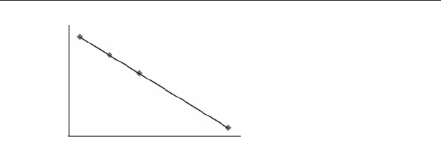
from it by using a regression line (Figure 16.1). This is another deliberate

example where the dependent variable is not caused by the independent

variable but is plausibly dependent on it.

A linear regression analysis gives an equation for a line that describes the

functional relationship between two variables and tests whether the statis-

tics that describe this line are signiﬁcantly diﬀerent from zero.

The simplest functional relationship between a dependent and independ-

ent variable is a straight line. Only two statistics, the intercept a (which is the

value of Y when X is zero) and the slope of the line b, are needed to uniquely

describe where that line occurs on a graph.

The position of any point on a straight line can be described by the equation:

¼ a þ bX

(16:1)

where a is the value of Y when X =0, and b is the slope of the line. For

example, the equation Y = 6 + 0.5X means “The Y value is 6 units plus half

the value of X.” Therefore, for this line, when X

=0,Y

= 6, and when X

=10,

= 11.

Simple linear regression analysis gives an equation for a straight line that

is the “best ﬁt” through a set of data points. It is very easy to obtain a and b if

all the points lie on a straight line. When the points are scattered, the

method for obtaining these statistics is also straightforward.

16.3 Calculation of the slope of the regression line

The slope of the regression line is the amount by which the value of Y

increases in relation to an increase in the value of X. For example, if an

Wt.% SiO

Temperature

Figure 16.1 An example of the use of regression. The eruption temperature

of a magma (the dependent variable) can be predicted by measuring its SiO

content (the independent variable). Thus the temperature is determined by

and easy to predict from the independent variable, but is not caused by it.

16.3 Calculation of the slope of the regression line 205

increase in the value of X by one unit is also accompanied by a one unit

increase in the value of Y, the slope of the line is 1.0. If, however, the value of Y

decreases by three units for every one unit increase in X then the slope is −3.0.

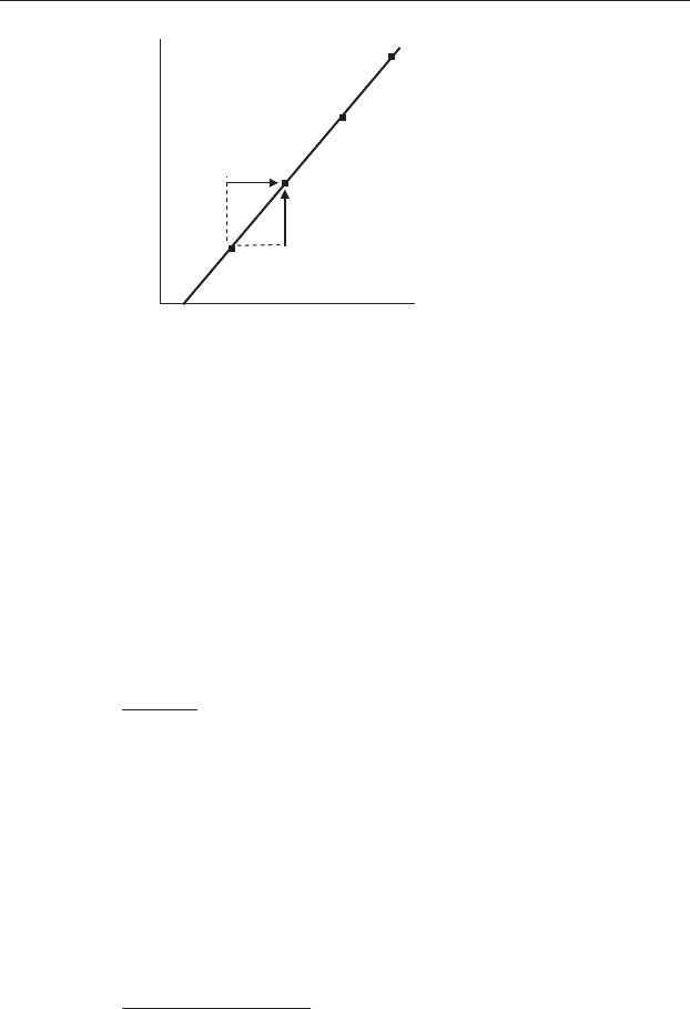
If all points lie along a straight line, you can calculate the slope by taking

any two points and using the equation:

b ¼

 Y

 X

(16:2)

that divides the relative change in Y by the relative change in X.

Equation (16.2) will not work for a set of points that are scattered. To

calculate the slope of the line of best ﬁt running through a set of scattered

points, a procedure is needed that gives the average slope, taking into

account the values for all of the points. The equation for calculating b, the

slope of the regression line, is:

b ¼

i¼1

ðX





XÞðY





YÞ

i¼1

ðX





XÞðX





XÞ

(16:3)

This is an extension of Equation (16.2). Instead of calculating the change in

X and Y from any two data points, Equation (16.3) calculates an average

slope using every point in the data set.

–

Figure 16.2 Calculation of the slope when all points lie along a straight line.

The vertical arrow shows the relative change in Y from Y

to Y

that occurs

with an increase in X from X

to X

shown by the horizontal arrow. For any

two points, Y

− Y

divided by X

− X

will give the slope, which in this case is

positive because Y increases as X increases and vice versa.

206 Linear regression

First, the means of X and Y are separately calculated. Next, for each data

point, the value of X minus its mean is multiplied by the value of Y minus its

mean, and these products are summed. This is the numerator of Equation

(16.3), which is then divided by the sum of each value of X minus its mean

and squared. It is easy to see how Equation (16.3) will give an appropriate

average value for the slope. The ﬁrst examples are for points that lie on

straight lines.

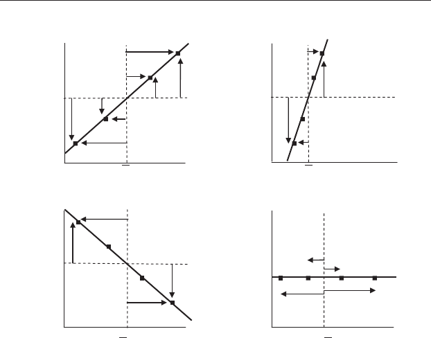
For a line with a slope of +1,asX increases by one unit from its mean,

the value of Y will also increase by one unit from its mean (and vice versa if

X decreases). The diﬀ erence between any value of X and its mean will always

be the same as the diﬀerence between any value of Y and its mean, so the

numerator and denominator of Equation (16.3) will be the same thus giving

a b value of 1.0 (Figure 16.3(a)).

For a line with a slope of +3,asX increases by one unit from its mean,

the value of Y will increase by three units from its mean (and vice versa if X

decreases). Therefore, the value of the numerator of Equation (16.3) will

always be three times the size of the denominator, no matter how many

points are included, thus giving a b value of 3.0 (Figure 16.3(b)).

For a line with a slope of − 1,asX increases by one unit from its mean,

the value of Y will decrease by one unit from its mean (and vice versa if X

decreases). Therefore the numerator of Equation (16.3) will give a total that

is the same magnitude but the negative of the denominator, thus giving a b

value of –1.0 (Figure 16.3(c)).

For a line with a slope of − 3, as X increases by one unit from its mean,

the value of Y will decrease by three units from its mean (and vice versa if X

decreases), so the numerator of Equation (16.3) will always have a negative

sign and be three times the value of the denominator, thus giving a b value

of –3.0.

Finally,

for a line

running parallel to the X axis, every value of Y





will be zero, so the total of the numerator of Equation (16.3) will also be

zero, thus giving a b value of zero (Figure 16.3(d)).

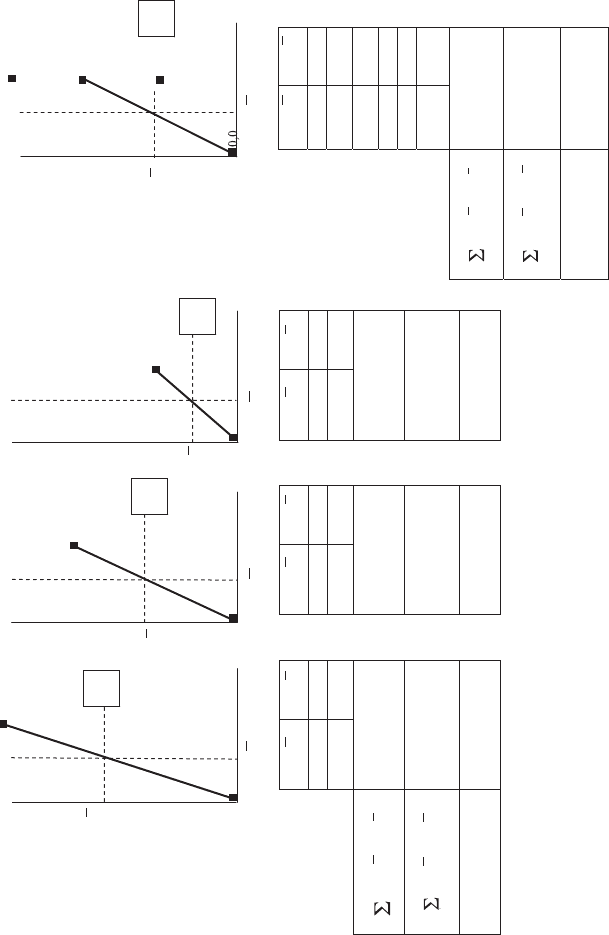
When the data are scattered, Equation (16.3) will also give the average

change in Y in relation to the increase in X. Figure 16.4 gives an example.

First, cases 16.4 (a), (b) and (c) show three lines, each of which has been

drawn through two data points. These lines have slopes of 3.0, 2.0 and 1.0

respectively, and the calculation of each b value is given in the box under the

graph. In Figure 16.4 (d) the six data points have been combined. Intuitively,

16.3 Calculation of the slope of the regression line 207

this group of six scattered points should have a slope of 2.0, because this is

the average of the slopes of the three lines shown in (a), (b) and (c). Equation

(16.3) gives this value.

16.4 Calculation of the intercept with the Y axis

The intercept of the regression line with the Y axis when X = 0 is easy to

calculate, using an extension of the formula for the regression line.

(a)

(b)

(c)

(d)

Figure 16.3 Examples of the use of Equation (16.3) to obtain the slope of

the regression line. Vertical arrows show Y





Y and horizontal arrows show





X. (a) For every point along a line with a slope of 1.0, Y





Y will be

the same magnitude and sign as X





X so Equation (16.3) will give a value of

1.0. (b) For every point along a line with a slope of 3.0, Y





Y will be the

same sign but three times greater than X





X so Equation (16.3) will give a

value of 3.0. (c) For every point along a line with a slope of –1.0, Y





Y will be

the same magnitude but the opposite sign to X





X so Equation (16.3) will

give a value of –1.0. (d) For a slope of zero, each value of Y





Y will be zero, so

Equation (16.3) will give a value of zero.

208 Linear regression

(a) (b) (c)

0,0 0,0 0,0

– X

– X )(Y

– Y )

– X )(X

– X )

– X X

– XY

– Y Y

– Y

4,8

4,4

X = 2

X = 2X = 2

4,12

22224

–4

–2

–2 –2

i = 1

(d)

4,12

4,8

4,4

–2

X = 2

Y X

–4

––

– X)(Y

– Y)

– X)(X

– X)

i = 1

Figure 16.4 Graphs (a), (b) and (c) show three lines of slope 3, 2 and 1 respectively, with two data points on each. The six points have been combined

in (d), and the line of best ﬁt through these would be expected to have a slope of 2.0. Use of Equation (16.3) givesthisappropriateaverageforb.

Box 16.1 Using regression to date geological samples

An important use of regression is the age dating of geological samples

using the radiometric decay of a parent isotope (P) to form a stable

daughter isotope (D). This relationship uses D as the dependent variable

(equivalent to Y in Equation (16.1)) and P as the independent one

(equivalent to X in Equation (16.1)):

D ¼ D

þðe

 1ÞP (16:4)

where D is the amount of daughter isotope present in the rock today, D

is the expected amount present when the rock cooled in the past, e is the

exponential, λ is the decay constant of the parent isotope, t is the age of

the sample and P is the amount of parent isotope present today. Parent–

daughter pairs with diﬀerent half-lives are useful in a range of geological

applications:

Decay reaction Half-life (years) Decay constant (/year)

C !

N t

1=2

¼ 5:73  10

l ¼ 1:2  10

4

K !

Ar t

1=2

¼ 1:3  10

l ¼ 5:81  10

11

Rb !

Sr t

1=2

¼ 4:86  10

l ¼ 1:42  10

11

147

Sm !

143

Nd t

1=2

¼ 1:06  10

l ¼ 6:54  10

12

238

U !

206

Pb t

1=2

¼ 4:4  10

l ¼ 1:55125  10

10

For example, the half-life of

C is only 5730 years, so after ~40 000

years there is not enough left to measure, therefore

C dating is most

useful for young rocks and biological remains. Conversely, ancient mete-

orites that date back billions of years to the beginning of the solar system

are usually dated using

238

U→

206

Pb.

If D is plotted against P for several crystals of a mineral from the same

rock, then the slope of the line of best ﬁt (termed an isochron) is equal to

λt

− 1, and the age of the rock, t, can be estimated.

One of the most useful systems in isotope geochemistry is the decay of

K (the parent isotope) to

Ar (the daughter). The isotope

Ar is quite

volatile when rocks are molten, so it can easily escape from a magma into

the atmosphere. When a rock crystallizes, however, the

Ar can no longer

escape and gets locked up in the crystal structures of the minerals, where it

accumulates as the

K in the rock continues to decay. This makes for a

210 Linear regression

Because

¼ a þ bX

(16:5 copied from 16:1)

then:



Y ¼ a þ b



X (16:6)

and this can be rearranged to give the value of a from:

a ¼



Y  b



X (16:7)

Statistical packages will do this as part of a regression analysis.

16.5 Testing the signi ﬁcance of the slope and the intercept

of the regression line

Although the equation for a regression line describes the functional rela-

tionship between X and Y, it does not show whether the slope of the line and

the intercept are signiﬁcantly diﬀerent from zero.

very useful geochronometer to tell us the crystallization age, because any

subsequent heating back to the liquid state will release all the

Ar. Thus, if

we measure the amounts of

Kand

Ar in a few feldspar crystals from a

rock, we can use the equations above to calculate the crystallization age of

the rock and the amount of

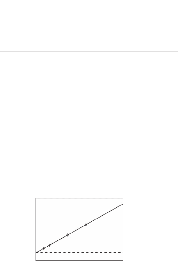
Ar in the original magma (Figure 16.5).

now

start

Isochron

Slope =(e

λt

–1)

now

Figure 16.5 A radiometric decay line for

K →

Ar as measured in four

feldspars from the same outcrop. The slope of this line can tell you the age, t, of

the rock because λ is known to be 0.581 × 10

–10

/yr as measured for this decay

reaction. The intercept estimates how much

K was present in the feldspars

when the rock ﬁrst cooled.

16.5 Testing the signiﬁcance 211

For a population, the equation of the line of best ﬁt is:

¼  þ X

(16:8)

but because earth scientists usually only have data for a sample, the pop-

ulation statistics α and β are only estimated by the sample statistics a and b,

so you need to test the null hypotheses that a and b are from a population

where α and β are zero. Please note that you will ﬁnd diﬀerent symbols for

the intercept and slope in some texts. Introductory texts generally use a and

b (and for a population, α and β) for the intercept and slope, but more

advanced texts use b

and b

for these two sample statistics and β

and β

for

the equivalent population statistics. Here we have used the same symbols as

most introductory texts for clarity.

16.5.1 Testing the hypothesis that the slope is signiﬁcantly

diﬀerent from zero

One method for testing whether the slope of a regression line is signiﬁcantly

diﬀerent from a slope of zero is very similar to the single-factor ANOVA

described in Chapter 10. A pictorial explanation is given in Figures 16.6

and 16.7.

Graphs of four regression lines are shown in Figure 16.6 together with a

horizontal line showing



Y, the average value of Y, which the regression line

will always cross. If there is no increase or decrease in the value of Y as X

increases, the regression line will have a slope of zero and be indistinguish-

able from the line showing



Y (Figure 16.6(a)). Nevertheless, samples taken

from a population where β is zero will, by chance, have values of b dis-

tributed around zero, often giving regression lines that are slightly tilted

upwards or downwards (Figure 16.6(b) and (c)). Finally, if there is a marked

increase or decrease in Y as X increases, the regression line will be strongly

tilted (e.g. a negative slope is shown in Figure 16.6(d)).

The amount by which the regression line is tilted from the horizontal can

be detected in the same way a single-factor ANOVA detects whether several

treatment means are all similar to the grand mean, or whether any are

signiﬁcantly displaced from it.

In Chapter 10 we described how a single-factor ANOVA calculates an F

ratio by dividing the mean square for treatment (i.e. treatment + error) by

the mean square for error only. If treatment has no eﬀect, the treatment

212 Linear regression