Stacey F.D., Davis P.M. Physics of the Earth
Подождите немного. Документ загружается.


//FS2/CUP/3-PAGINATION/SDE/2-PROOFS/3B2/9780521873628APX03.3D
–
457
– [457–461] 13.3.2008 10:52AM
Appendix C
Spherical harmonic functions
Spherical harmonic analysis may be regarded
as the adaption of Fourier analysis to a spherical
surface. It is therefore a convenient way of rep-
resenting and analysing physical phenomena
and properties that are distributed over the
Earth’s surface. However, spherical harmonics
haveamorefundamentalsignificancethanmere
convenience. They are solutions of Laplace’s
equation, which is obeyed by potential fields
(gravity, magnetism) outside the sources of the
fields, and of the seismic wave equation in spher-
ical geometry. Thus spherical harmonic repre-
sentations are appropriate for the Earth’s
gravitational and magnetic fields and for free
oscillations. Somewhat different procedures
and normalizations are applied in the different
sub-disciplines of geophysics. A statement of the
mathematical properties of ‘spherical harmonic
functions is given in Chapter 3 of Sneddon
(1980). Chapman and Bartels (1940, Vol.2) give
details of the application to geomagnetism and
the discussion by Kaula (1968) is useful, particu-
larly in the application to gravity.
Laplace’s equation is most familiar in Cartesian
coordinates,
r
2
V ¼
@
2
V
@x
2
þ
@
2
V
@y
2
þ
@
2
V
@z
2
¼ 0: (C:1)
Rewritten in spherical polar coordinates it is
r
2
V ¼
1
r
2
@
@r
r
2
@V
@r
þ
1
r
2
sin
@
@
sin
@V
@
þ
1
r
2
sin
2
@
2
V
@l
2
¼ 0; ðC:2Þ
where V is the potential describing a particular
field. The origin (r ¼0) is normally the centre
of the Earth. is the angle with respect to the
chosen coordinate axis, commonly but not nec-
essarily the Earth’s rotational axis, in which case
it is co-latitude (908 latitude) and l is longitude,
measured from a convenient reference (the
Greenwich meridian if not otherwise specified).
The wave equation can be written in similar
form:
@
2
V
@t
2
¼ c
2
r
2
V; (C:3)
where c is wave speed and V is the potential whose
derivative in any direction gives the component
of displacement in that direction. By imposing
spherical geometry on this equation, we see that
the solutions describing free oscillations of the
Earth have the surface patterns of the spherical
harmonic solutions of Laplace’s equation (C.2).
Equation (C.2) is rendered tractable by assum-
ing a separation of variables, that is V is the
product of separate functions of r, and l. This
procedure is justified by the fact that it yields
solutions of the form
V ¼ r
l
; r
lþ1ðÞ
hi
cos ml; sin ml½P
lm
cos ðÞ: (C:4)
The square brackets give alternative solutions. l
and m are integers with m l, and P
lm
() satisfies
the equation
1
2
d
2
P
d
2
2
dP
d
þ llþ 1ðÞ
m
2
1
2
P ¼ 0:
(C:5)

//FS2/CUP/3-PAGINATION/SDE/2-PROOFS/3B2/9780521873628APX03.3D
–
458
– [457–461] 13.3.2008 10:52AM
This reduces to Legendre’s equation for the
case m ¼0, for which there is no variation in V
with longitude. Equation (C.5) with m 6¼0is
Legendre’s associated equation. Considering
first the special case m ¼0, solutions of Eq. (C.5)
have the form
P
l0
ðÞ¼
1
2
l
l!
d
l
d
l
2
1
l
hi
; (C:6)
where the multiplying factor 1/2
l
l! does not
affect the solution but normalizes the function
so that P
l0
(1) ¼þ1. Sneddon (1980) refers to this
as Rodrigue’s formula. The functions P
l0
(cos ),
for the case m ¼0, are the Legendre polynomials,
normally written with the second subscript
omitted, P
l
(cos ). If convenient, latitude, ,
may be used instead of co-latitude, , by substi-
tuting ¼cos ¼sin . Explicit expressions for
the first few P
l
(cos ) are given in the m ¼0
column of Table C.1.
In putting m ¼0, we restrict the solutions to
the description of potentials with rotational sym-
metry. These are zonal harmonics. As in Eq. (C.4),
a potential that is expressed in zonal harmonics
is written as a sum of terms, each of which is
a power of r, with the Legendre polynomials
appearing in the coefficients and representing
the latitude variations. In geophysical problems
it is convenient to make the coefficients dimen-
sionally equal by normalizing r to the Earth’s
radius, a.Thus
V ¼
1
a
X
1
l¼0
C
l
a
r
lþ1
þC
0
l
r
a
l
P
l
cos ðÞ; (C:7)
where the C
l
are constant coefficients represent-
ing sources of potential inside the surface con-
sidered and the C
l
0
are due to external sources.
Equation (C.7) is a sum of terms with the form of
Eq. (C.4) with m ¼0.
The derivation of MacCullagh’s formula for the
gravitational potential due to a distributed mass
with a slight departure from spherical symmetry
can be extended to obtain a more complete solu-
tion,withtheformofEq.(C.7).If,insteadofter-
minating the expansion of Eq. (6.4) at terms in 1/r
2
,
we continue to higher powers in 1/r, the coeffi-
cients are Legendre polynomials, i.e.
1 þ
s
r
2
2
s
r
cos w
1=2
¼
X
1
l¼0
s
r
l
P
l
cos wðÞ: (C:8)
Applying this expansion to the potential in
Eq. (6.3), we obtain an infinite series with the
Table C.1 Legendre polynomials P
l
(cos ) and associated polynomials, p
lm
(cos ). Numerical
factors convert P
lm
to p
m
l
m ¼0 m ¼1
l ¼ 0 11 – –
1 cos
ffiffiffi
3
p
sin
ffiffiffi
3
p
2
1
2
3 cos
2
1
ffiffiffi
5
p
3cos sin
ffiffiffiffiffiffiffiffi
5=3
p
3
1
2
5 cos
3
3 cos
ffiffiffi
7
p
3
2
5 cos
2
1
sin
ffiffiffiffiffiffiffiffi
7=6
p
4
1
8
35 cos
4
30 cos
2
þ 3
ffiffiffi
9
p
5
2
7 cos
3
3 cos
sin
ffiffiffiffiffiffiffiffiffiffi
9=10
p
m ¼2 m ¼3 m ¼4
l ¼0 –– – – – –
1––––––
2 3 sin
2
ffiffiffiffiffiffiffiffiffiffi
5=12
p
–– – –
3 15 cos sin
2
ffiffiffiffiffiffiffiffiffiffi
7=60
p
15 sin
3
ffiffiffiffiffiffiffiffiffiffiffiffiffi
7=360
p
––
4
15
2
7 cos
2
1
sin
2
ffiffiffiffiffiffiffiffiffiffi
1=20
p
105 cos sin
3
ffiffiffiffiffiffiffiffiffiffiffiffiffi
1=280
p
105 sin
4
ffiffiffiffiffiffiffiffiffiffiffiffiffiffiffi
1=2240
p
458 AP P EN D I X C
//FS2/CUP/3-PAGINATION/SDE/2-PROOFS/3B2/9780521873628APX03.3D
–
459
– [457–461] 13.3.2008 10:52AM
form of Eq. (6.1) in which the coefficients J
l
rep-
resent the multipole moments of the mass
distribution.
Now consider the more general case of a
potential that does not have rotational symme-
try, so that m 6¼0 in Eqs. (C.4) and (C.5). By differ-
entiation and substitution we can show that
Eq. (C.5) has solutions
P
lm
ðÞ¼1
2
m=2
d
m
d
m
P
l0
ðÞ½
¼
1
2
l
l!
1
2
m=2
d
lþm
d
lþm
2
1
l
hi
: (C:9)
These are the associated Legendre polyno-
mials, or Ferrer’s modified version (Sneddon,
1980), introduced to avoid factors (1)
m/2
in the
original. It is a straightforward matter to calcu-
late the first few functions directly from Eq. (C.9),
but a more convenient polynomial form is
P
lm
cos ðÞ¼
sin
m
2
l
X
Int lmðÞ=2½
t¼0
1ðÞ
t
2l 2tðÞ!
t! l tðÞ! l m 2tðÞ!
cos
lm2t
:
(C:10)
The upper limit of this summation is the integ-
ral part of [(l m)/2], ignoring the extra 1/2 for
odd values of (l m). Explicit forms for the low-
est degrees (l) and orders (m) are listed in
Table C.1.
The general expression for potential as a sum
of spherical harmonics is
V ¼
1
a
X
1
l¼0
X
l
m¼0
C
lm
a
r
lþ1
þC
0
lm
r
a
l
cos ml
þ S
lm
a
r
lþ1
þS
0
lm
r
a
l
sin ml
8
>
>
>
>
<
>
>
>
>
:
9
>
>
>
>
=
>
>
>
>
;
P
lm
cos ðÞ; ðC: 11Þ
which is simply a sum of terms with the form of
Eq. (C.4). As with Eq. (C.7) the unprimed coeffi-
cients refer to internal sources, which have van-
ishing influence at r !1, and the primed
coefficients are attributable to external sources.
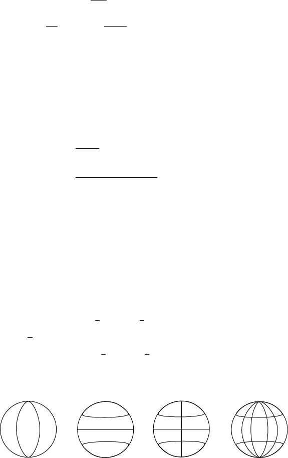
The general surface patterns of spherical har-
monics can be seen by considering Eqs. (C.4) or
(C.11) and (C.10). Around any complete (3608)
line of latitude (at fixed ) there is a sinusoidal
variation with l, crossing 2m meridians where
the function vanishes. The latitude variation is
less obvious, but examination of Eq. (C.10) shows
that down any selected meridian, that is over
1808 from pole to pole, there are (l m) values
of latitude where the function vanishes. Thus l
gives the total number of nodal lines on one
hemisphere and is a measure of the fineness of
the structure represented; m determines the dis-
tribution of the total between lines of latitude
and longitude (Fig. C.1). For m ¼0 they are all
latitudinal and for m ¼l they are all longitudinal.
The upper limit of m is l, as can be seen in
Eq. (C.9) because when (
2
1)
l
is differentiated
(l þm) times the derivative vanishes for m > l.
For the purposes of this text we are inter-
ested mainly in the terms with unprimed coef-
ficients in Eq. (C.11). These terms all decrease
with increasing distance from the origin (and
from the internal source of the potential) and
the rate of decrease increases with l. The low
harmonic degrees become increasingly domi-
nant at greater distances. Conversely, extrapolat-
ing downwards from surface observations, the
higher harmonic degrees become increasingly
prominent. The harmonics are expressing the
obvious principle that fine details at depth are
difficult to discern at the surface because of the
spatial attenuation.
A common feature of the terms in a Fourier
series and the Legendre and associated polyno-
mials is that they are orthogonal. This means
_
_
+
_
_
_
_
_
_
_
_
_
_
_
_
_
+
++
+
+
+
+
+
+
+
+
+
+
+
lm = 22 lm = 30 lm = 41 lm = 64
FIG U R E C.1. Examples of
spherical harmonics. m ¼0 gives
zonal harmonics, m ¼l gives
sectoral harmonics and general
cases, 0 < m < l, are known as
tesseral harmonics.
SPHERICAL HARMONIC FUNCTIONS 459

//FS2/CUP/3-PAGINATION/SDE/2-PROOFS/3B2/9780521873628APX03.3D
–
460
– [457–461] 13.3.2008 10:52AM
that the integral over a sphere of any product
vanishes,
ð
2p
0
ð
1
1
P
lm
ðÞP
l
0
m
0
ðÞcos ml; sin ml½:
cos m
0
l; sin m
0
l
½
d dl ¼ 0; ðC:12Þ
(C:12)
unless both l
0
¼l and m
0
¼m. This means that in
a harmonic analysis of a complete data set over
a spherical surface the coefficients of the har-
monic series are independent and errors are not
introduced by truncating the series. However, the
calculated coefficients are affected by truncation
when discrete or irregularly spaced data are used,
as is normally the case.
In some treatments of Legendre polynomials
the subscript n is used in place of l. Here n is
reserved for a further development that appears
in the study of free oscillations – a harmonic radial
variation. Free oscillations are classified in
Section 5.3 according to the values of three
integers; thus
n
S
m
l
and
n
T
m
l
denote spheroidal
and torsional oscillati ons, respectively, where
l, m represent variations on a spherical surface,
as for P
lm
(cos y)cos ml,andn is the number o f
internal spherical surfaces that are nodes of the
motion.
The numerical factors in the associated poly-
nomials defined by Eqs. (C.9) and (C.10) increase
rapidly with m; to make the coefficients in a
harmonic analysis relate more nearly to the
physical significance of the terms they repre-
sent, various normalizing factors are used. The
one that has been employed in most recent anal-
yses of the geoid and must be favoured for gen-
eral adoption is the ‘fully normalized’ function
p
m
l
cos ðÞ¼2
m;0
2l þ 1ðÞ
l mðÞ!
l þ mðÞ!
1=2
P
lm
cos ðÞ;
(C:13)
which is so defined that
1
4p
ð
2p
0
ð
1
1
p
m
l
cos ðÞsin ml; cos ml½
2
d cos ðÞdl ¼ 1;
(C:14)
that is, the mean square value over a spherical
surface is unity. Note that the factor (2
m
,
0
)
in Eq. (C.12) is unity if m ¼0, but (2
m
,
0
) ¼2
if m 6¼0 because the factor sin ml; cos ml
½
2
in
Eq. (C.14) introduces a factor 1/2. (There is no
alternative sin ml term if m ¼0.) The coefficients
of a spherical harmonic expansion referred
to the normalized coefficients, p
m
l
, are distin-
guished by a bar:
C
m
l
; S
m
l
. Thus
V ¼
1
a
X
1
l¼0
X
l
m¼0
C
m
l
a
r
lþ1
þC
0
m
l
a
r
l
cos ml
þ
S
m
l
a
r
lþ1
þS
0
m
l
r
a
l
sin ml
8
>
>
>
>
<
>
>
>
>
:
9
>
>
>
>
=
>
>
>
>
;
p
m
l
cos ðÞ: ðC:15Þ
The spherical harmonics used in geomagnetism
apply no normalization to the zonal harmonics
(m ¼0), but bring the sectoral and tesseral har-
monics into line with the zonal harmonics of
the same degree by applying the normalizing
factor 2
m;0
l mðÞ!= l þ mðÞ!
1=2
.
It is of interest to consider the spherical har-
monic expansions of some simple surface pat-
terns that are subject to analytical represent-
ation. Thus, if we consider the equation for the
surface of an oblate ellipsoid of equatorial radius
a and eccentricity e,
r ¼ a 1 þ
e
2
1 e
2
sin
2
1=2
; (C:16)
and expand in powers of e to e
6
or flatten f ¼
(1 c/a)tof
3
and zonal harmonics to P
6
, we have
r
a
¼ 1
e
2
6
11
20
e
4
103
1680
e
6
þ
e
2
3
5
42
e
4
3
56
e
6
P
2
þ
3
35
e
4
þ
57
770
e
6
P
4
5
231
e
6
P
6
; ðC:17Þ
r
a
¼ 1
f
3
f
2
5
13
105
f
3
þ
2
3
f
1
7
f
2
þ
1
21
f
3
P
2
þ
12
35
f
2
þ
96
385
f
3
P
4
40
231
f
3
P
6
: ðC:18Þ
Note that the P
2
term alone does not represent an
ellipsoidal surface, although for the Earth the
ellipticity is sufficiently slight that expansion
to e
4
, f
2
,P
4
suffices.
460 AP P EN D I X C

//FS2/CUP/3-PAGINATION/SDE/2-PROOFS/3B2/9780521873628APX03.3D
–
461
– [457–461] 13.3.2008 10:52AM
Ifweconsiderasinglesurfacespikeof
negligible lateral dimensions, we obtain equal
coefficients for all unnormalized zonal harmonics
or amplitudes proportional to (2l þ1)
1/2
in fully
normalized harmonics. For a pair of opposite
points the even terms follow the same pattern,
but the odd terms vanish. Another geometrically
simple case is a great circle line source, which also
gives vanishing odd terms, but even coefficients
(fully normalized) varying as
C
l
¼ð1Þ
l=2
1=2
l
ðl=2Þ!
½
2
ð2l þ 1Þ
1=2
: (C:19)
The values of this function oscillate in sign with
amplitudes very close to 1.12/(2l þ1), except
C
0
¼1.
SPHERICAL HARMONIC FUNCTIONS 461

//FS2/CUP/3-PAGINATION/SDE/2-PROOFS/3B2/9780521873628APX04.3D
–
462
– [462–463] 13.3.2008 10:51AM
Appendix D
Relationships between elastic moduli
of an isotropic solid
Table D.1 Elastic moduli (see Section 10.2)
K E l
K, K
3K 2
6K þ 2
9K
3K þ
K
2
3
K þ
4
3
K, K
3Kð1 2Þ
2ð1 þ Þ
3K(1 2)
3K
1 þ
3Kð1 Þ
ð1 þ Þ
K,EK
3KE
9K E
1
2
E
6K
E
3Kð3K EÞ
9K E
3Kð3K þ EÞ
9K E
K,l K
3
2
ðK lÞ
l
3K l
9KðK lÞ
3K l
l 3K 2l
K, K
3
4
ð KÞ
3K
3K þ
9Kð KÞ
3K þ
1
2
ð3K Þ
,
2ð1 þ Þ
3ð1 2Þ
2(1 þ)
2
1 2
2ð1 Þ
ð1 2Þ
,E
E
3ð3 EÞ
E
2
1
E
ðE 2Þ
3 E
ð4 EÞ
3 E
,l
l þ
2
3
l
2ðl þ Þ
ð3l þ 2Þ
l þ
llþ2
,
4
3
2
2ð Þ
ð3 4Þ
2
,E
E
3ð1 2Þ
E
2ð1 þ Þ
E
E
ð1 þ Þð1 2Þ
Eð1 Þ
ð1 þ Þð1 2Þ
,l
lð1 þ Þ
3
lð1 2Þ
2
lð1 þ Þð1 2Þ
l lð1 Þ
,
ð1 þ Þ
3ð1 Þ
ð1 2Þ
2ð1 Þ
ð1 þ Þð1 2Þ
1
1

//FS2/CUP/3-PAGINATION/SDE/2-PROOFS/3B2/9780521873628APX04.3D
–
463
– [462–463] 13.3.2008 10:51AM
Table D.1 (cont.)
K E l
E,l
E þ 3l þ p
6
E 3l þ p
4
p E l
4l
E l
E l þ p
2
E,
3 E þ q
6
E þ 3 q
8
E þ q
4
E
E þ q
4
l,
1
3
ð2l þ Þ
1
2
ð lÞ
l
l þ
ð2l þ Þð lÞ
l þ
l
p ¼
ffiffiffiffiffiffiffiffiffiffiffiffiffiffiffiffiffiffiffiffiffiffiffiffiffiffiffiffiffiffiffiffi
E
2
þ 2E l þ 9l
2
p
; q ¼
ffiffiffiffiffiffiffiffiffiffiffiffiffiffiffiffiffiffiffiffiffiffiffiffiffiffiffiffiffiffiffiffiffiffiffi
E
2
10E þ 9
2
q
Note: for mathematical convenience it is sometimes assumed that there is only one independent
modulus, with l ¼ and therefore K ¼5/3, ¼3 ¼9K/5, ¼1/4. This is referred to as a
Poisson solid, but it is not a good approximation for rocks and becomes increasingly
unsatisfactory with increasing pressure.
ELASTIC MODULI OF AN ISOTROPIC SOLID 463
//FS2/CUP/3-PAGINATION/SDE/2-PROOFS/3B2/9780521873628APX05.3D
–
464
– [464–468] 13.3.2008 10:51AM
Appendix E
Thermodynamic parameters and
derivative relationships
Tables E.2 and E.3 present a compact summary of
thermodynamic derivatives in a form convenient
for geophysical applications. Individual entries
have no meaning; they must be taken in pairs
sothat,forexample,tofind(qT/qP)
S
look down
the constant S column and take the ratio of
entries for qT and qP,thatisT/ K
S
. An arbitrary
mass m of material is assumed, so that m
appears in many of the entries. Table E.2 is
complete for the eight primary parameters.
Any one of them may be differentiated with
respect to any other one with any third one
held constant. The results a re represented in
terms of the same parameters plus a set of first
derivative properties, , K
T
, K
S
, C
V
, C
P
and .
Table E.3 extends the constant T, P, V and S
columns to derivatives of these first derivative
properties, using a set of second derivative
parameters, K
0
T
, K
0
S
,
T
,
S
, C
0
T
, C
0
S
and q,defined
inTableE.1.Therearenumerousalternative
forms for many of the Table E.3 entries, the
usefulness of which depends on particular
applications. Substitutions may be made using
relationships in Table E.4. A few derivatives of
products and third derivatives have been found
useful and are also listed.
The compact collection of thermodynamic
derivatives in Tables E.2 and E.3 follows an
idea, started by Bridgman (1914), that is much
more useful than generally realized. Bridgman’s
original compilation was difficult to use because
it related derivatives to one another and not to
familiar parameters, as in the tables presented
here. Also, some confusion arose from errors
that were copied in later compilations and not
corrected for another 80 years (Dearden, 1995).

//FS2/CUP/3-PAGINATION/SDE/2-PROOFS/3B2/9780521873628APX05.3D
–
465
– [464–468] 13.3.2008 10:51AM
Table E.1 Thermodynamic notation and definitions (note that parameters V, S, U, H, F
and G refer to arbitrary mass, m, but C
V
and C
P
refer to unit mass)
Specific heat, constant PC
P
¼(T/m)(@S/@T)
P
constant VC
V
¼(T/m)(@S/@T)
V
C
0
S
¼(@ ln C
V
/@ ln V)
S
; C
0
T
¼(@ ln C
V
/@ ln V )
T
Helmholtz free energy F ¼U TS
Gibbs free energy G ¼U TS þPV
Enthalpy H ¼U þPV
Bulk modulus, adiabatic K
S
¼V(@P/@V)
S
K
0
S
¼(@K
S
/qP)
S
; K
00
S
¼(@K
0
S
/@P)
S
isothermal K
T
¼V(@P/@V)
T
K
0
T
¼(@K
T
/@P)
T
; K
00
T
¼ (@K
0
T
/@P)
T
Pressure P
q ¼(@ ln g/@ ln V)
T
¼(@ ln(gC
V
)/@ ln V)
S
q
S
¼(@ ln g/@ ln V)
S
¼q C
0
S
Heat Q
Entropy S ¼
Ð
dQ=T
Temperature T
Internal energy U
Volume V
Volume expansion coefficient ¼(1/V)(qV/qT)
P
Gr
¨
uneisen parameter ¼K
T
/C
V
¼K
S
/C
P
Anderson–Gr
¨
uneisen parameter, adiabatic
S
¼(1/)(@ ln K
S
/@T )
P
¼(@ ln(T/C
P
)/@ ln V)
S
isothermal
T
¼(1/)(@ ln K
T
/@T )
P
¼(@ ln /@ ln V)
T
Density ¼m/V
l ¼(@ ln q/@ ln V)
T
THERMODYNAMIC PARAMETERS AND DERIVATIVE RELATIONSHIPS 465

//FS2/CUP/3-PAGINATION/SDE/2-PROOFS/3B2/9780521873628APX05.3D
–
466
– [464–468] 13.3.2008 10:51AM
Table E.2 First order derivatives of thermodynamic parameters
Differential
element
Constant
TPVS U H F G
@T –11TPK
T
T 1 TP 1
@P K
T
/V – K
T
¼C
V
K
S
C
V
(K
S
P) C
P
K
T
(S/VþP) S/V
@V 1 V – VmC
V
V(1 þ1/) S V S/K
T
@S K
T
¼C
V
mC
P
/TmC
V
/T – mC
V
P/TmC
P
/TmC
V
(P/TS/V) mC
P
/T S
@U K
T
T PmC
P
VP mC
V
PV – mC
P
PV
(1 þ1/)
mC
V
P SK
T
T
þSP
mC
P
TS PV
þSP/K
T
@H K
T
(1 T) mC
P
mC
V
(1 þ) K
S
VmC
V
[P(1 þ)
K
S
]
– SK
T
(1 T)
þmC
V
P(1 þ)
mC
P
þS(1 T)
@F P SVP SPVTS C
V
(TS PV)
PS
S(1 T)
PV(1 þ1/)
– S (1 P/K
T
)
PV
@G K
T
S S þK
T
VK
S
V TS mC
V
(TS/V
þP K
S
) PS
S(1 T)
mC
P
S(K
T
P)
þPVK
T
–