Simon Benninga. Financial Modelling 3-rd edition

Подождите немного. Документ загружается.

358 Chapter 13

Solving the equation for the vector of expected portfolio returns, this

expression means that an efﬁ cient portfolio must solve the following

equation:

Expected

portfolio

returns

Variance-

covariance

matrix

⎡

⎣

⎢

⎤

⎦

⎥

⎡⎡

⎣

⎢

⎤

⎦

⎥

⎡

⎣

⎢

⎤

⎦

⎥

∗

Efficient

portfolio

proportions

Normalizing

ffactor

Risk-free

rate

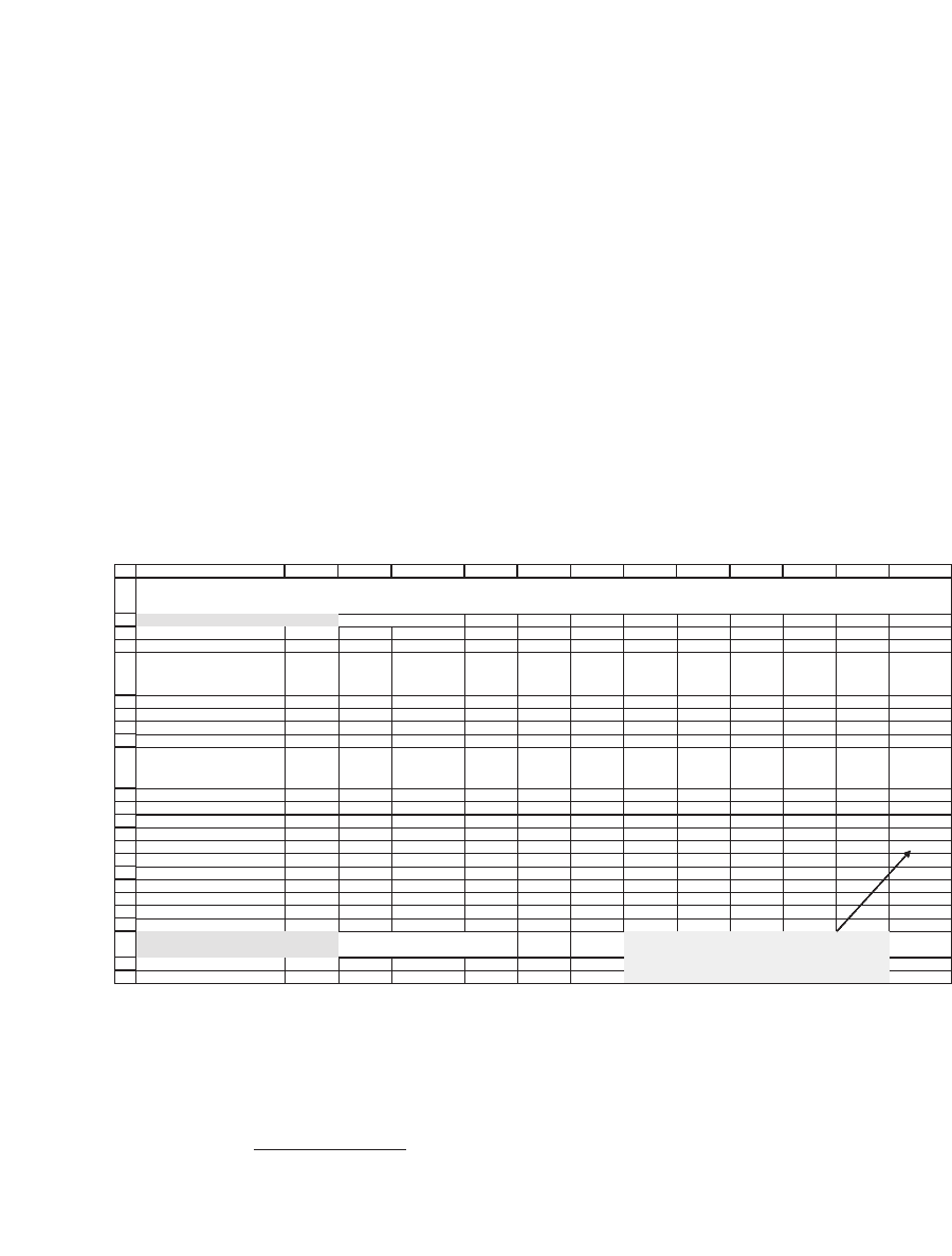
Joanna assumes that, in the absence of any additional knowledge or

opinions about the market, the current market weights of the portfolio

indicate the efﬁ ciency weights. She estimates that the expected bench-

mark return over the next month will be 1 percent and uses this estima-

tion to set the normalizing factor.

Solving the ﬁ rst part of the latter equation (without the normalizing

factor) gives the following:

ABCDEFGHIJKL

Anticipated benchmark return 1.00% <

=12%/12

Current t-bill rate 0.40%

General

Motors

Home

Depot

International

Paper

Hewlett-

Packard

HPQ

Altria

American

Express

AXP

Alcoa

Aluminum

DuPont

Merck

MRK

MMM

Equity value 16.85 73.98 15.92 88.37 153.33 65.66 28.16 38.32 79.51 60.9

Benchmark proportions 2.71% 11.91% 2.56% 14.23% 24.69% 10.57% 4.53% 6.17% 12.80% 9.81%

Variance-covariance matrix

GM HD IP HPQ MO AXP AA DD MRK MMM

Without

normalizing

factor

GM 0.0116 0.0030 0.0023 0.0041 0.0013 0.0032 0.0046 0.0018 0.0010 0.0014 0.27%

HD 0.0030 0.0071 0.0018 0.0042 0.0022 0.0033 0.0045 0.0020 0.0002 0.0018 0.31%

IP 0.0023 0.0018 0.0039 0.0031 0.0001 0.0023 0.0043 0.0021 0.0012 0.0016 0.18%

HPQ 0.0041 0.0042 0.0031 0.0117 0.0025 0.0048 0.0060 0.0033 0.0019 0.0022 0.46%

MO 0.0013 0.0022 0.0001 0.0025 0.0076 0.0016 0.0018 0.0009 0.0007 0.0008 0.31%

AXP 0.0032 0.0033 0.0023 0.0048 0.0016 0.0041 0.0037 0.0019 0.0011 0.0014 0.27%

AA 0.0046 0.0045 0.0043 0.0060 0.0018 0.0037 0.0091 0.0040 0.0018 0.0024 0.37%

DD 0.0018 0.0020 0.0021 0.0033 0.0009 0.0019 0.0040 0.0038 0.0016 0.0019 0.21%

MRK 0.0010 0.0002 0.0012 0.0019 0.0007 0.0011 0.0018 0.0016 0.0065 0.0005 0.18%

MMM 0.0014 0.0018 0.0016 0.0022 0.0008 0.0014 0.0024 0.0019 0.0005 0.0031 0.16%

Check: The expected return

of the benchmark?

0.29% <

{=MMULT(B7:K7,M11:M20)}

SUPER DUPER BENCHMARK PORTFOLIO--WHAT DOES THE MARKET THINK?

No normalizing factor

Cells M11:M20 contain the array formula

{=MMULT(B11:K20,TRANSPOSE(B7:K7)+B3)}

Note that given the weights in row 7, the expected benchmark return is

0.29 percent per month as opposed to the 1 percent per month posited

by Joanne (cell B2). To achieve this expected benchmark returns we

multiply row 7 by a normalizing factor.

4. One percent per month is equivalent to estimating an annual expected benchmark

return of 12 percent.

359 The Black-Litterman Approach to Portfolio Optimization

Benchmark

portfolio

returns

Variance-

covariance

matri

⎡

⎣

⎢

⎤

⎦

⎥

Benchmark

portfolio

proportions

Normalizin

⎡

⎣

⎢

⎤

⎦

⎥

⎡

⎣

⎢

⎤

⎦

⎥

∗

factor

Risk-free

rate

Variance-

covariance

matrix

⎡

⎣

⎢

⎤

⎦

⎥

nnchmark

portfolio

proportions

Expected benchmark re

⎡

⎣

⎢

⎤

⎦

⎥

∗

tturn Risk-free rate

Benchmark

portfolio

proportions

−

⎡

⎣

⎢

⎤

⎦

⎥

VVariance-

covariance

matrix

Benchmark

portfolio

propor

⎡

⎣

⎢

⎤

⎦

⎥

ttions

The normalizing factor

⎡

⎣

⎢

⎤

⎦

⎥

⎛

⎝

⎜

⎞

⎠

⎟

⎛

⎝

⎜

⎞

⎠

⎟

↑



Risk-free

rate

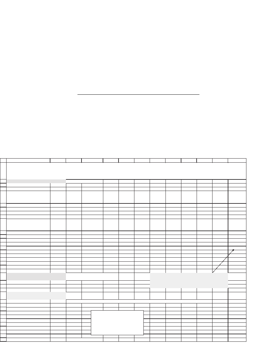
This procedure is illustrated in the next spreadsheet:

ABCDEFGHIJKL

Anticipated benchmark return 1.00% <

=12%/12

Current t-bill rate 0.40%

General

Motors

Home

Depot

International

Paper

Hewlett-

Packard

HPQ

Altria

American

Express

AXP

Alcoa

Aluminum

DuPont

Merck

MRK

MMM

Equity value 16.85 73.98 15.92 88.37 153.33 65.66 28.16 38.32 79.51 60.9

Benchmark proportions 2.71% 11.91% 2.56% 14.23% 24.69% 10.57% 4.53% 6.17% 12.80% 9.81%

Variance-covariance matrix

GM HD IP HPQ MO AXP AA DD MRK MMM

With

normalizing

factor

GM 0.0116 0.0030 0.0023 0.0041 0.0013 0.0032 0.0046 0.0018 0.0010 0.0014 0.96%

HD 0.0030 0.0071 0.0018 0.0042 0.0022 0.0033 0.0045 0.0020 0.0002 0.0018 1.05%

IP 0.0023 0.0018 0.0039 0.0031 0.0001 0.0023 0.0043 0.0021 0.0012 0.0016 0.77%

HPQ 0.0041 0.0042 0.0031 0.0117 0.0025 0.0048 0.0060 0.0033 0.0019 0.0022 1.36%

MO 0.0013 0.0022 0.0001 0.0025 0.0076 0.0016 0.0018 0.0009 0.0007 0.0008 1.05%

AXP 0.0032 0.0033 0.0023 0.0048 0.0016 0.0041 0.0037 0.0019 0.0011 0.0014 0.97%

AA 0.0046 0.0045 0.0043 0.0060 0.0018 0.0037 0.0091 0.0040 0.0018 0.0024 1.17%

DD 0.0018 0.0020 0.0021 0.0033 0.0009 0.0019 0.0040 0.0038 0.0016 0.0019 0.84%

MRK 0.0010 0.0002 0.0012 0.0019 0.0007 0.0011 0.0018 0.0016 0.0065 0.0005 0.77%

MMM 0.0014 0.0018 0.0016 0.0022 0.0008 0.0014 0.0024 0.0019 0.0005 0.0031 0.73%

Check: The expected return

of the benchmark?

1.00% <

{=MMULT(B7:K7,M11:M20)}

GM 2.71% <

{=MMULT(MINVERSE(B11:K20),M11:M20-B3)/SUM(MMULT(MINVERSE(B11:K20),M11:M20-B3))}

HD 11.91%

IP 2.56%

HPQ 14.23%

MO 24.69%

AXP 10.57%

AA 4.53%

DD 6.17%

MRK 12.80%

MMM 9.81%

Sum of proportions 100.0% <

=SUM(B27:B36)

SUPER DUPER BENCHMARK PORTFOLIO--WHAT DOES THE MARKET THINK?

We multiply row 7 by a normalizing factor

The expected returns make the benchmark optimal

Cells M11:M20 contain the array formula

{=(MMULT(B11:K20,TRANSPOSE(B7:K7))*(B2-

B3)/MMULT(B7:K7,MMULT(B11:K20,TRANSPOSE(B7:

K7))))+B3}

Additional check:

Optimal portfolio

Note that Chapter 9 optimization on

the expected returns in cells

M11:M20 and the variance-

covariance matrix produces the

market weights as the optimal

portfolio.

360 Chapter 13

We have performed an additional check in the spreadsheet by deriving

the optimal portfolio given the current T-bill rate of 0.40 percent and the

expected returns in M11 : M20. This should give us back the benchmark

proportions in row 7—and it does!

13.5 Black-Litterman Step 2: Introducing Opinions—What Does Joanna Think?

Having made two assumptions—(1) that the benchmark is efﬁ cient

and (2) that the expected benchmark return is 1 percent per month—

Joanna has derived the expected returns for each of the benchmark

components (cells M11 : M20). We are now ready to introduce Joanna’s

opinions about asset returns. The rough idea is that if she disagrees with

a market return, she can use the optimization procedure from Chapter

9 to derive a portfolio whose proportions differ from those of the

benchmark.

We have to be careful, however: Because asset returns are correlated,

any opinion Joanna has about one asset’s returns will translate to an

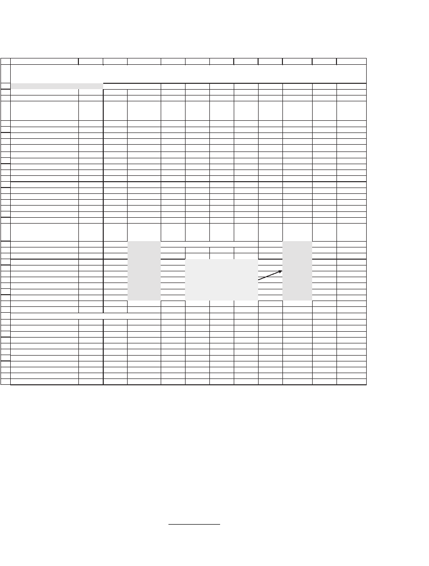
opinion about all other asset returns. To illustrate this point, suppose that

Joanna thinks that the return on GM will be 1.1 percent over the next

month instead of the market opinion of 0.96 percent. Then this assump-

tion translates to the following picture:

361 The Black-Litterman Approach to Portfolio Optimization

The δ introduced in column B of the preceding ﬁ gure indicates

Joanna’s deviation from the Black-Litterman base case. In this example,

Joanna thinks that GM will have a monthly return 0.14 percent higher

than the market’s return of 0.96 percent (cell B24). Because of the co-

variance between asset returns, this change means that the HD return

she expects is 1.11 percent:

HD, opinion adjusted HD, market

HD, GM

Cov( )

Var

=+ =

()

.δ 1 11%%

ABCDEFGHIJK

Anticipated benchmark return 1.00% <

=12%/12

Current t-bill rate 0.40%

General

Motors

Home

Depot

International

Paper

Hewlett-

Packard

HPQ

Altria

American

Express

AXP

Alcoa

Aluminum

DuPont

Merck

MRK

MMM

Equity value 16.85 73.98 15.92 88.37 153.33 65.66 28.16 38.32 79.51 60.9

Benchmark proportions 2.71% 11.91% 2.56% 14.23% 24.69% 10.57% 4.53% 6.17% 12.80% 9.81%

Variance-covariance matrix

GM HD IP HPQ MO AXP AA DD MRK MMM

GM 0.0116 0.0030 0.0023 0.0041 0.0013 0.0032 0.0046 0.0018 0.0010 0.0014

HD 0.0030 0.0071 0.0018 0.0042 0.0022 0.0033 0.0045 0.0020 0.0002 0.0018

IP 0.0023 0.0018 0.0039 0.0031 0.0001 0.0023 0.0043 0.0021 0.0012 0.0016

HPQ 0.0041 0.0042 0.0031 0.0117 0.0025 0.0048 0.0060 0.0033 0.0019 0.0022

MO 0.0013 0.0022 0.0001 0.0025 0.0076 0.0016 0.0018 0.0009 0.0007 0.0008

AXP 0.0032 0.0033 0.0023 0.0048 0.0016 0.0041 0.0037 0.0019 0.0011 0.0014

AA 0.0046 0.0045 0.0043 0.0060 0.0018 0.0037 0.0091 0.0040 0.0018 0.0024

DD 0.0018 0.0020 0.0021 0.0033 0.0009 0.0019 0.0040 0.0038 0.0016 0.0019

MRK 0.0010 0.0002 0.0012 0.0019 0.0007 0.0011 0.0018 0.0016 0.0065 0.0005

MMM 0.0014 0.0018 0.0016 0.0022 0.0008 0.0014 0.0024 0.0019 0.0005 0.0031

Expected benchmark returns,

no opinions

Analyst

opinion,

delta

Returns

adjusted for

opinions

Optimized

benchmark

proportions

Portfolio

benchmark,

no opinions

0.96% 0.14% GM 1.10% <

{=A24:A33+MMULT(B38:K47,B24:B33)} 5.19% GM 2.71%

1.05% 0.00% HD 1.11% 8.23% HD 11.91%

0.77% 0.00% IP 0.86% 7.60% IP 2.56%

1.36% 0.00% HPQ 1.41% 6.60% HPQ 14.23%

1.05% 0.00% MO 1.07% 20.72% MO 24.69%

0.97% 0.00% AXP 1.08% 22.17% AXP 10.57%

1.17% 0.00% AA 1.24% -1.98% AA 4.53%

0.84% 0.00% DD 0.91% 10.67% DD 6.17%

0.77% 0.00% MRK 0.79% 9.54% MRK 12.80%

0.73% 0.00% MMM 0.79% 11.26% MMM 9.81%

Tracking factors: in each row i Cov(r

) is divided by Var(r

)

GM HD IP HPQ MO AXP AA DD MRK MMM

GM 1.0000 0.2589 0.1999 0.3540 0.1153 0.2788 0.3920 0.1555 0.0829 0.1169

HD 0.4257 1.0000 0.2603 0.5934 0.3119 0.4635 0.6376 0.2834 0.0250 0.2501

IP 0.5985 0.4738 1.0000 0.7940 0.0222 0.5954 1.0994 0.5306 0.3056 0.4063

HPQ 0.3527 0.3594 0.2642 1.0000 0.2162 0.4145 0.5097 0.2791 0.1665 0.1878

MO 0.1769 0.2909 0.0114 0.3328 1.0000 0.2096 0.2351 0.1158 0.0884 0.1046

AXP 0.7843 0.7927 0.5595 1.1704 0.3845 1.0000 0.8956 0.4624 0.2556 0.3270

AA 0.5006 0.4950 0.4690 0.6533 0.1957 0.4066 1.0000 0.4404 0.1938 0.2625

DD 0.4820 0.5343 0.5496 0.8687 0.2342 0.5097 1.0694 1.0000 0.4327 0.5067

MRK 0.1483 0.0272 0.1826 0.2991 0.1032 0.1626 0.2715 0.2497 1.0000 0.0741

MMM 0.4437 0.5772 0.5151 0.7156 0.2588 0.4412 0.7802 0.6202 0.1571 1.0000

Cells J24:J33 contain the array

formula

{=MMULT(MINVERSE(B11:K20),D2

4:D33-

B3)/SUM(MMULT(MINVERSE(B11:K

20),D24:D33-B3))}

ADJUSTING THE BENCHMARK FOR AN ANALYST'S OPINION

In this example the only opinion is about GM

362 Chapter 13

IP, opinion adjusted IP, market

IP, GM

Cov( )

Var( )

=+ =

086.%%

and so on.

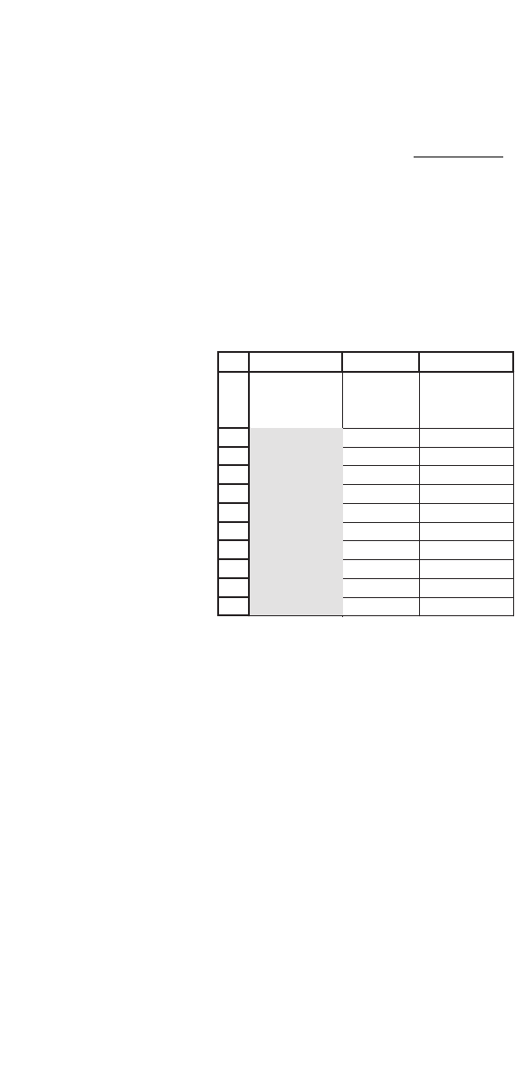
The newly optimized portfolio is given in cells J24 : J33. Joanna’s

opinion about GM has dramatically changed the portfolio composition

from its benchmark weights (L24 : L33):

JKL

Optimized

benchmark

proportions

Portfolio

benchmark,

no opinions

5.19% GM 2.71%

8.23% HD 11.91%

7.60% IP 2.56%

6.60% HPQ 14.23%

20.72% MO 24.69%

22.17% AXP 10.57%

-1.98% AA 4.53%

10.67% DD 6.17%

9.54% MRK 12.80%

11.26% MMM 9.81%

Notice that Joanna’s positive opinion about GM returns has, predict-

ably, increased the proportion of GM in her portfolio. But the opinion

about GM has also affected all the other portfolio weights—increasing

the weight on AXP, decreasing the weight on AA, . . . .

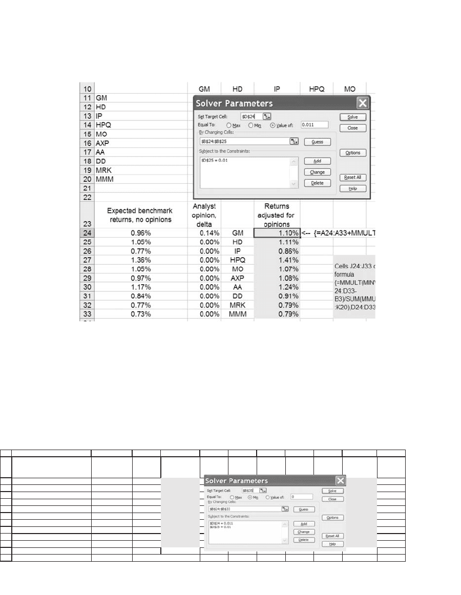
13.5.1 Two or More Opinions

If Joanna has two or more opinions, the situation becomes more

difﬁ cult. Suppose, for example, that she believes the GM return will be

1.10 percent instead of its market return of 0.96 percent and the

HD return will be 1 percent instead of its market return of 1.05

percent. Using Solver we can ﬁ nd a solution for δ

and δ

that gives

an opinion-adjusted return of 1.10 percent for GM and 1.00 percent

for HD:

363 The Black-Litterman Approach to Portfolio Optimization

EDCBA FGH I J

Expected benchmark returns,

no opinions

Analyst

opinion,

delta

Returns

adjusted for

opinions

Optimized

benchmark

proportions

0.96% 0.18% GM 1.10% <-- {=A24:A33+MMULT(B39:K48,B24:B33)} 8.92% GM

1.05% -0.10% HD 1.00% 5.36% HD

0.77% 0.01% IP 0.82% 8.19% IP

1.36%

-0.01% HPQ

1.36% 12.01% HPQ

1.05% -0.02% MO 1.02% 22.96% MO

0.97% -0.01% AXP 1.00% 14.49% AXP

1.17% -0.01% AA 1.19% 2.33% AA

0.84% -0.01% DD 0.85% 6.36% DD

0.77% 0.02% MRK 0.80% 13.05% MRK

0.73% -0.01% MMM 0.72% 6.32% MMM

Sum of squared deltas 4.32684E-06 <-- {=SUM(B24:B33^2)}

Cells J24:J33 contain the array

formula

{=MMULT(MINVERSE(B11:K20),D2

4:D33-

B3)/SUM(MMULT(MINVERSE(B11:K

20),D24:D33-B3))}

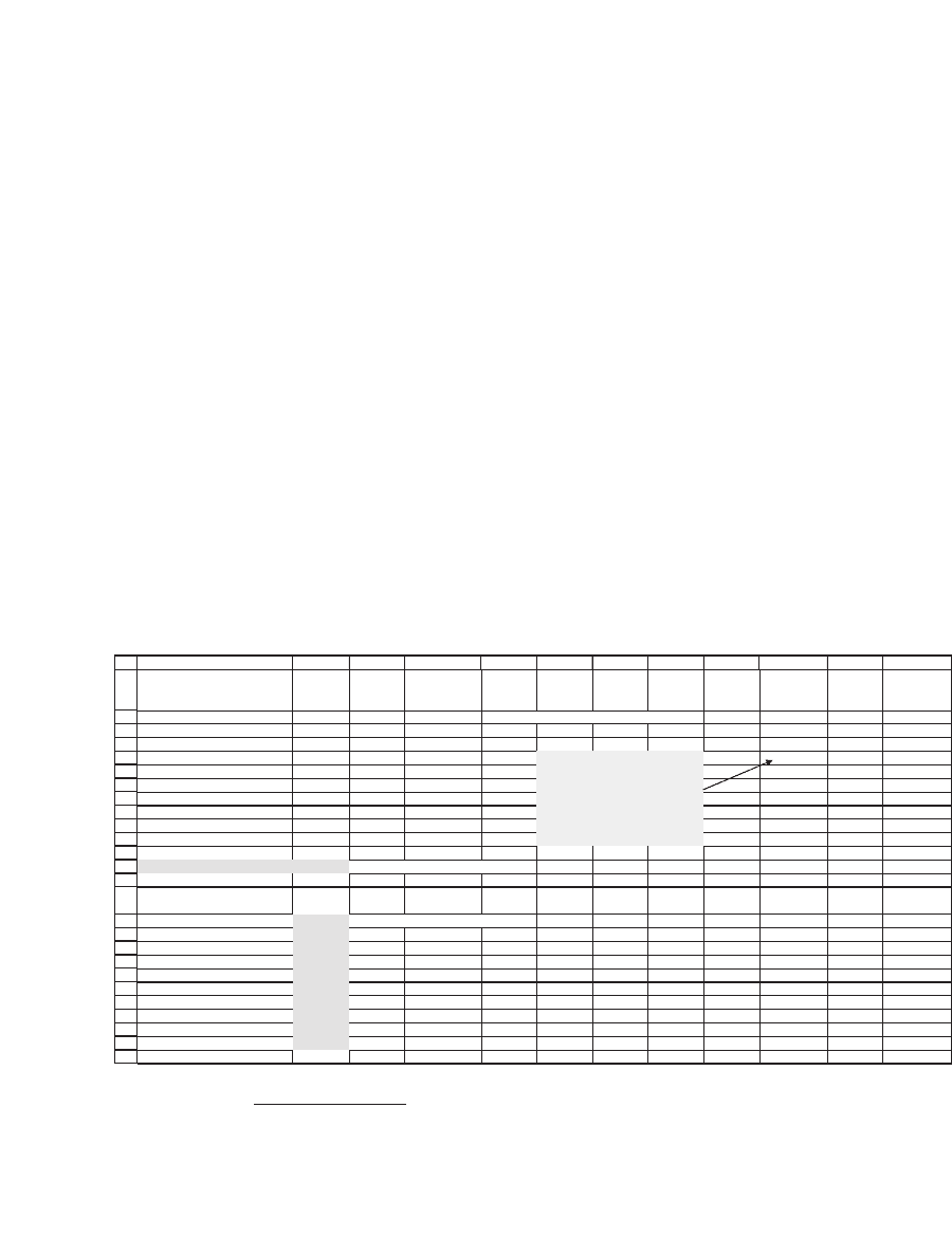
Note The philosophically inclined reader might well ask what an

“opinion” really is. In this example we have limited the deltas to be only

about GM and HD. However, suppose we allow deltas for other assets;

then we get a whole class of “opinions” that ﬁ t the bill of having E(r

)

= 1.10 percent and E(r

) = 1.00 percent. For example, if we are willing

to allow ds for all the assets, we could ask Solver for a minimal set of

divergent opinions ( ) that gives Joanna’s two expected returns for GM

and HD:

We achieved this result by using Solver:

364 Chapter 13

In the preceding spreadsheet clip, we have solved for the minimal squared

deltas that give the requisite opinions about GM and HD.

13.5.2 Do You Believe Your Opinions?

Do we really believe our own opinions? Do we actually have conﬁ dence

in what we believe? There is a whole theory of Bayesian adjustments to

our beliefs, which is adumbrated in Theil (1971).

An application to port-

folio modeling can be found in Black and Litterman (1991) and other

associated papers. This author ﬁ nds these papers dauntingly complicated

and difﬁ cult to implement. A simpler approach to the conﬁ dence ques-

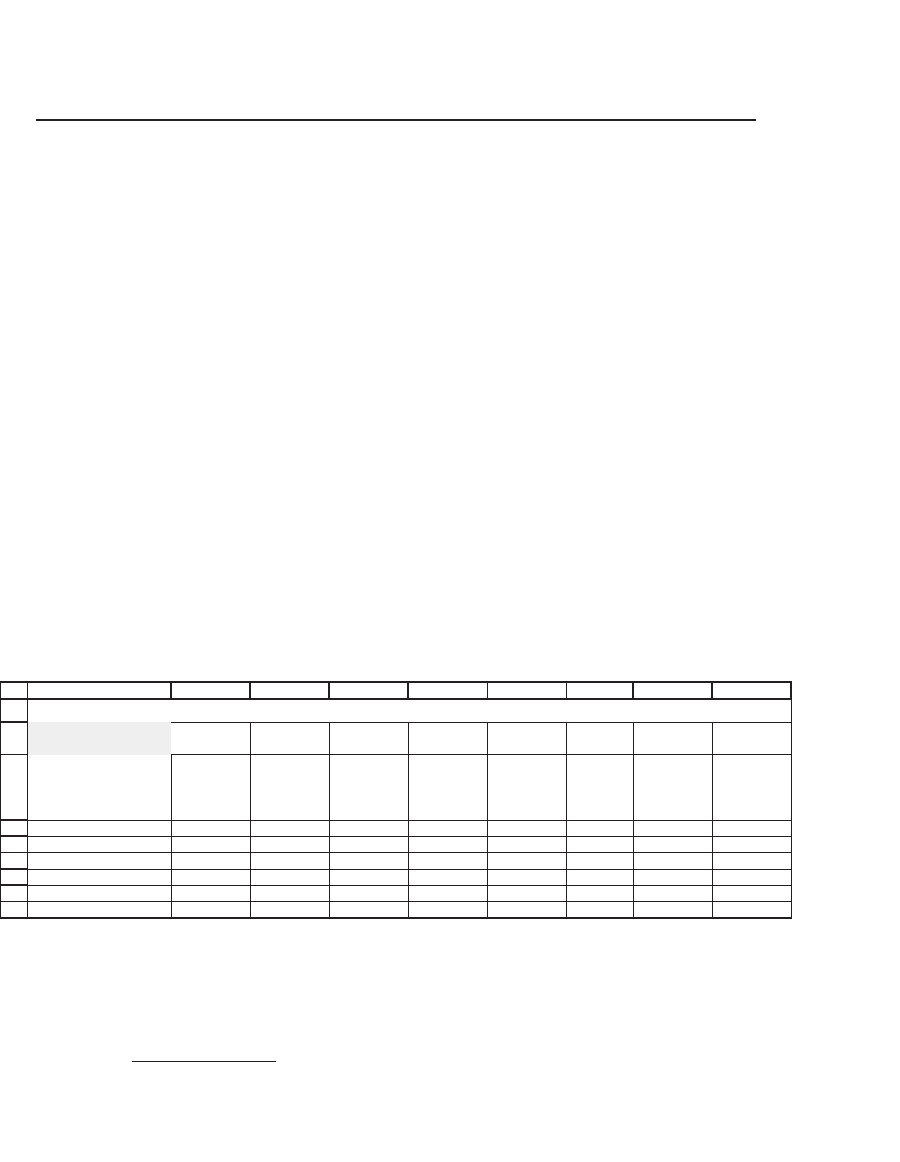
tion is to form a portfolio based on a convex combination of the market

weights and the opinion-adjusted weights:

Portfolio proportions Market weights

Opinion-adjuste

=−∗ +∗()1 γγ

dd weights

where γ is our degree of conﬁ dence in our opinions. Here is an applica-

tion to our last example:

ABCDEFGHIJK

Expected benchmark returns,

no opinions

Analyst

opinion,

delta

Returns

adjusted for

opinions

Optimized

benchmark

weights

Benchmark

weights, no

opinions

0.96% 0.17% 1.10% <

{=A24:A33+MMULT(B56:K65,B24:B33)} 8.32% GM 2.71%

1.05% -0.12% 1.00% 3.52% HD 11.91%

0.77% 0.00% 0.82% 7.13% IP 2.56%

1.36% 0.00% 1.37% 11.25% HPQ 14.23%

1.05% 0.00% 1.05% 23.56% MO 24.69%

0.97% 0.00% 1.01% 16.41% AXP 10.57%

1.17% 0.00% 1.20% 2.07% AA 4.53%

0.84% 0.00% 0.86% 7.72% DD 6.17%

0.77% 0.00% 0.79% 11.53% MRK 12.80%

0.73% 0.00% 0.74% 8.50% MMM 9.81%

, opinion confidence

0.60 <

Weight attached to analyst opinion

Opinion and confidence-

adjusted portfolio

GM 6.08% <

=(1-$B$35)*L24+$B$35*J24

HD 6.87%

IP 5.31%

HPQ 12.44%

MO 24.01%

AXP 14.08%

AA 3.06%

DD 7.10%

MRK 12.04%

MMM 9.02%

Sum of weights 100.00%

Cells J24:J33 contain the array

formula

{=MMULT(MINVERSE(B11:K20),D2

4:D33-

B3)/SUM(MMULT(MINVERSE(B11:K

20),D24:D33-B3))}

5. Note that this vector of deltas is not unique. If we replace cell B35 by the sum of the

absolute values of delta, we will get a different set of deltas (see exercises to this

chapter).

6. Theil, Henri. 1971. Principles of Econometrics. New York: Wiley and Sons.

365 The Black-Litterman Approach to Portfolio Optimization

13.6 Implementing Black-Litterman on an International Portfolio

We end this chapter by implementing the BL model on data for ﬁ ve

international indices.

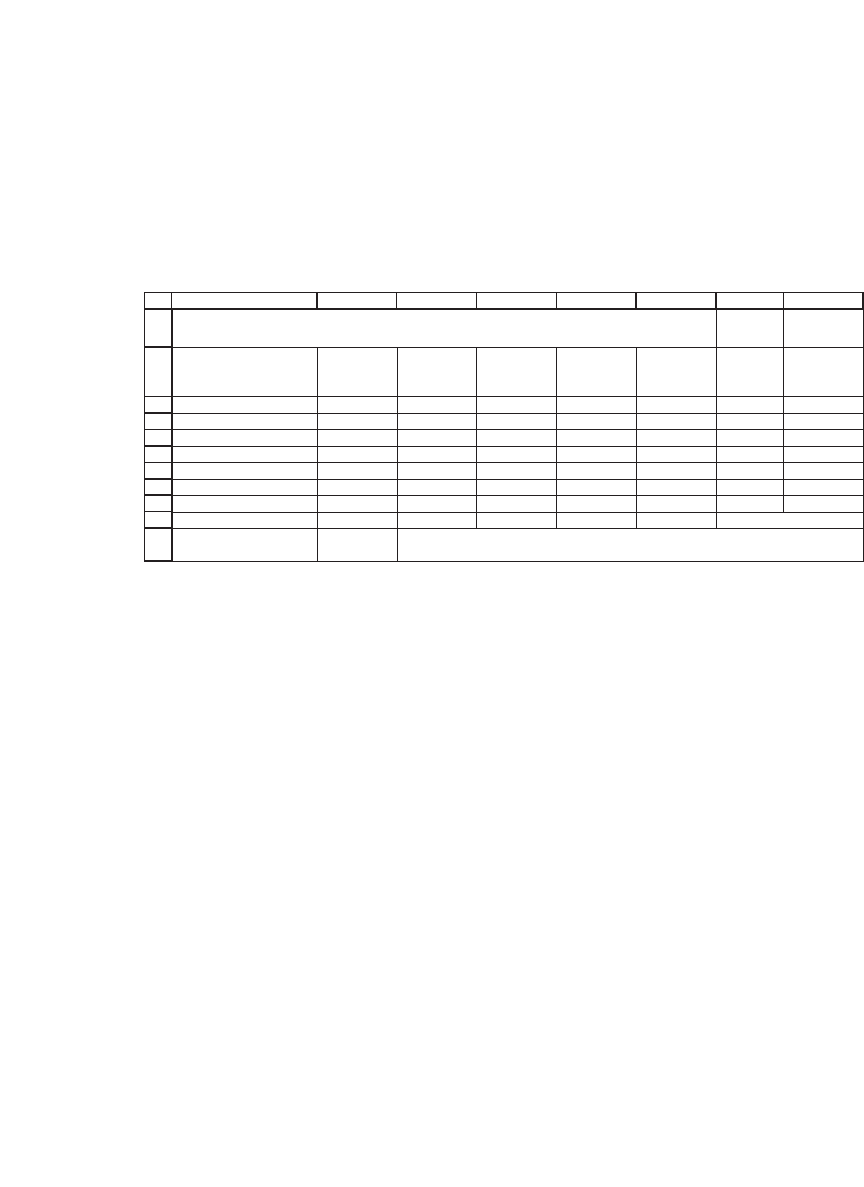
The spreadsheet that follows gives data on ﬁ ve

major world stock market indices:

1. The S&P 500, a value-weighted index of the 500 largest U.S. stocks.

2. The MSCI World ex-US index: The Morgan Stanley Capital Interna-

tional (MSCI) World ex-US index comprises 21 developed countries

based on GDP per capita.

3. The Russell 2000 index: The Russell 3000 Index is market cap weighted

and captures about 98 percent of the investable U.S. marketplace. The

Russell 2000 Index consists of the 2,000 smallest companies in the Russell

3000 Index.

4. The MSCI Emerging Markets index: The Morgan Stanley Capital

International (MSCI) Emerging Markets index consists of indexes for

26 emerging economies.

5. The LB Global Aggregate index: This Lehman Brothers index covers

the most liquid portion of the global investment-grade ﬁ xed-rate bond

market, including government, credit, and collateralized securities.

ABCDEFGH

5 YEARS ENDING

DEC05

Correlation S&P 500

MSCI

World ex-

Russell

2000

MSCI

Emerging

LB Global

Aggregate

Weight

Standard

deviation

S&P 500

1.0000 0.8800 0.8400 0.8100 -0.1600 24% 14.90%

MSCI World ex-US 0.8800 1.0000 0.8300 0.8700 0.0700 26% 15.60%

Russell 2000

0.8400 0.8300 1.0000 0.8300 -0.1400 3% 19.20%

MSCI Emerging

0.8100 0.8700 0.8300 1.0000 -0.0500 3% 21.00%

LB Global Aggregate

-0.1600 0.0700 -0.1400 -0.0500 1.0000 44% 5.80%

100%

INDEX DATA, 2001-2005

Column H gives the weights on the index in a composite portfolio as of

the end of December 2005, and column I gives the standard deviation of

each index component.

7. I thank Steven Schoenfeld of Northern Trust for providing me with the data and some

suggestions.

366 Chapter 13

13.6.1 The Variance-Covariance Matrix

We ﬁ rst use the wonders of the Excel array functions (see Chapter 34)

to compute the variance-covariance matrix for the ﬁ ve indexes:

ABCDEFG

Variance-covariance

matrix

S&P 500

MSCI

World ex-

Russell

2000

MSCI

Emerging

LB Global

Aggregate

S&P 500 0.0222 0.0205 0.0240 0.0253 -0.0014

MSCI World ex-US 0.0205 0.0243 0.0249 0.0285 0.0006

Russell 2000 0.0240 0.0249 0.0369 0.0335 -0.0016

MSCI Emerging 0.0253 0.0285 0.0335 0.0441 -0.0006

LB Global Aggregate -0.0014 0.0006 -0.0016 -0.0006 0.0034

Checks

First row of var-cov 0.0222 0.0205 0.0240 0.0253 -0.0014 <-- =I4*I8*F4

Standard deviation of

composite

8.72% <

{=SQRT(MMULT(MMULT(TRANSPOSE(H4:H8),B14:F18),H4:H8))}

Variance-covariance matrix: cells contain formula

{=I4:I8*TRANSPOSE(I4:I8)*B4:F8}

The strange formula, I4 : I8*TRANSPOSE(I4 : I8)*B4 : F8, in the cells

B14 : F19 is composed of two parts:

•

I4 : I8*TRANSPOSE(I4 : I8) multiplies the column vector I4 : I8 times

its transpose. This is equivalent to multiplying

MSCI World

Russell

MSCI Emerging

LB Global

500

2000

⎡

⎣

⎢

⎤⎤

⎦

⎥

∗

σσ σ σ σ

SP MSCI World Russell MSCI Emerging LB Glob500 2000 aal

[]

Which—in the wonderful world of array functions—gives a matrix of the

covariances:

σσ

MSCI World SP

LB Global SP

SP MSCI World

500



SSCI World

LB Global MSCI World

SP Russell

SP L

500 2000

500

σσ

…

……

BB Global

LB Global

⎡

⎣

⎢

⎤

⎦

⎥

367 The Black-Litterman Approach to Portfolio Optimization

•

Multiplying the preceding by the matrix of correlations B4 : F8 gives

the variance-covariance matrix.

•

Of course the whole array formula I4 : I8*TRANSPOSE(I4 : I8)*B4 : F8

is entered with [Ctrl] + [Shift] + [Enter].

In rows 21 and 22 we perform two checks on our computation: Row

21 contains brute-force computations of the ﬁ rst row of the variance-

covariance matrix—just to make sure our array formula works as adver-

tised. In cell B22 we compute the standard deviation of the ﬁ ve-index

portfolio using their relative weights.

ABCDEF

Risk-free rate 5.00%

Expected return on

S&P 500

12.00%

Black-Litterman implied returns

S&P 500

12.00% <-- {=MMULT(B14:F18,H4:H8)*(B26-

B12)/INDEX((MMULT(B14:F18,H4:H8)),1,1)+B12}

MSCI World ex-US

13.66%

Russell 2000

14.22%

MSCI Emerging

16.20%

LB Global aggregate

1.30%

The Black-Litterman implied expected returns are based on three

assumptions:

•

The weighted portfolio of the ﬁ ve indexes is mean-variance optimal.

•

The anticipated risk-free rate is 5 percent.

•

The expected return of the S&P 500 index is 12 percent.

Given these assumptions, the expected returns on the ﬁ ve-index

portfolio are given in cells B29 : B33. Note the array formula given in

these cells:

=∗MMULT(B14:F18,H4:H8) (B26-B12)/INDEX

((MMULT(B14:F18,H4:H8))),1,1) B12+

This formula uses the expected return on the S&P 500 to normalize the

returns. It is equivalent to