Sha W., Malinov S. Titanium Alloys: Modelling of Microstructure, Properties and Applications
Подождите немного. Документ загружается.


331
14
Neural network models and applications
in phase transformation studies
Abstract: This chapter provides two examples of using artificial neural
network (ANN) modelling for predicting, respectively, the β -transus and
time–temperature–transformation diagrams as functions of alloying elements
for binary and commercial titanium alloys. The first part of this chapter
shows some comparisons of the ANN model developed with Thermo-Calc
predictions. The second part of the chapter gives indications of how
individual alloying elements will shift the C-curve and affect the martensite
start temperature. This information will be of interest to persons working in
the field of phase transformation of titanium alloys.
Key words: neural network, TTT diagrams, phase transformation, β-transus
temperature, MatLab.
14.1 β-transus temperature
The β-transus (β
tr
) temperature is one of the most important characteristics
of titanium alloys. It is usually taken as the basic reference point when a
treatment is designed. Therefore, it is very desirable to determine this
temperature for a given alloy accurately, especially for some near-α alloys
whose processing window is narrow. Traditionally, β
tr
is determined
experimentally by the phase disappearing method. In this method, samples
are first aged to precipitate α phase. They are then reheated to various
temperatures separated by 15 °C intervals, held for 15 min, followed by
water quenching. The β
tr
of the alloy studied is then no more than 15 °C
above the highest temperature for which α phase is detected metallographically.
The 15 °C interval can be further reduced to get a more accurate estimation
of β
tr
. β
tr
is strongly dependent on alloy chemistry, so the measurement
should be examined at a number of location points if the product to be
assessed is of large scale. Such procedures are both time-consuming and
costly. Since the most important influential factor on the value of β
tr
is the
alloy chemistry, it is of great importance to quantify the relationship between
the β
tr
temperature and the amount of alloying elements.
Multiple linear regression analysis has been adopted in the past, to quantify
the β
tr
temperature as a function of the alloying amounts of various elements.
This type of analysis was usually developed to deal with a certain type of
alloy within a certain composition range. Sometimes, results from different
researchers were contradictory to each other. Moreover, linear models always
suffer from the drawback that interactions between alloying elements cannot
Titanium alloys: modelling of microstructure332
be taken into account. Artificial neural network (ANN) modelling, which
employs non-linear regression analysis tools, can overcome this disadvantage,
and has found a variety of applications in materials science.
Since little prior knowledge of the physical background of the processes
is required when using an ANN, and to a lesser extent when developing an
ANN, this method can dramatically benefit the industry, as industrial
metallurgists often have to solve their problems without full comprehension
of the scientific background. This section will demonstrate using the artificial
neural network modelling technique to construct a quantitative model for
titanium alloys that can predict the β
tr
temperature of a titanium alloy when
the alloy chemistry is known. The β
tr
temperature from thermodynamic
calculation will also be shown, to compare with the results from ANN
modelling. The influence of the database scale for ANN modelling on the
model performance will also be discussed.
14.1.1 Model description
An artificial neural network provides a way of using examples of a target
function to find the coefficients that make a certain mapping function
approximate the target function as closely as possible. Each node (also called
neuron) in the input layer represents in the network the value of one independent
variable. The nodes in the hidden layer are only for computation purposes.
Each of the output nodes computes one dependent variable. More details
about the principles of ANN modelling can be found in Chapter 13. A three-
layer (one input, one hidden and one output) ANN with sigmoid transfer
functions in the hidden layer can map any function of practical interest, so a
three-layer neural network model is used in this section.
Input and output parameters
The selection of the property-related parameters, or input parameters, is
based on the physical background of how the target property is determined.
Omitting the parameters which are not important benefits model development
and simplifies further application. Because β
tr
is mainly the function of alloy
chemistry, the input for the present model is the chemical composition of the
titanium alloy, whereas the output is the β
tr
temperature.
Database construction and analysis
Construction of a reliable database is the first critical step. The data set for
β
tr
temperature modelling includes 200 input–output data pairs collected
from open literature, industrial data from Timet, and the ‘Titanium and its
alloys’ database compiled from data supplied by the member companies of

Neural network models and applications 333
Titanium Information Group and Titanium Development Association and
developed by MATUS Databases Engineering Information Co. Ltd. It consisted
of nine input variables, and one output variable. The input variables are the
concentrations of elements Al, Cr, Fe, Mo, Sn, Si, V, Zr and O. As very few
alloys contain Ta and Ni, their influences are taken into account by converting
their concentration to [Mo]
eq
([Mo]
eq
= [Mo] + [Ta]/5 + 1.25[Ni] + …),
instead of considering them as individual input variables. The output variable
is the β
tr
temperature. Table 14.1 summarises some features of the data set in
a statistical term.
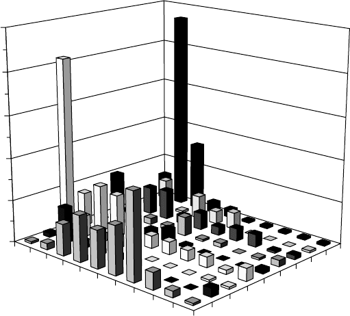
The distribution of the input values within specific concentration intervals
is another very important characteristic of the data set, since it shows intervals
where we can achieve higher or lower accuracy of training and prediction.
The distribution here is presented as a form of histogram in ten equally
spaced containers between minimal and maximal values of the alloying
elements (Fig. 14.1). The model is expected to be more accurate at the places
of high data density.
Training
Many parameters can be altered in order to obtain a well-trained model, an
important one being the training algorithm. It has become standard for some
years to train artificial neural networks by the backpropagation method. The
term backpropagation refers to the manner in which the gradient is computed
for non-linear multilayer networks. The early standard algorithm consists of
assigning a random initial set of weights to each synapse of the neural
network, then presenting the data inputs, one set at a time, and adjusting the
weights with the aim of reducing the corresponding output error. This is
Table 14.1
Statistical analysis of the input and output variables for the β-transus
model (concentration in wt. %)
Variable Number of alloys Min. Max. Mean Standard
containing this deviation
element
Al 135 0 9.6 3.22 2.64
Cr 48 0 11.2 0.92 2.10
Fe 109 0 5.0 0.29 0.67
Mo 100 0 16.08 2.66 4.00
Sn 42 0 11.0 0.66 1.59
Si 34 0 0.5 0.03 0.09
V 64 0 20.16 2.51 4.59
Zr 41 0 11.0 0.81 1.84
O 152 0 0.9 0.12 0.13
β-transus (°C) – 670 1080 892.2 100.4
Titanium alloys: modelling of microstructure334
repeated for each set of data, and then the complete cycle is repeated until an
acceptably low value of the sum of squares error is achieved. Such an algorithm
is usually both inefficient and unreliable, requiring many iterations to converge,
if it converges at all. Therefore, a number of variations of the standard
algorithm have been developed, based on other optimisation techniques,
with a variety of computation and storage advantages. These are detailed in
The Math Works, Inc. product, Neural Network Toolbox for MatLab. One of
the most popular algorithms is Bayesian regularisation (TRAINBR). TRAINBR
is a MatLab command for the function. PREMNMX, POSTMNMX,
TRAMNMX, TANSIG, PURELIN, and NEWGRNN, which appear later,
are also MatLab commands. The Bayesian regularisation (BR) algorithm
usually results in ANN models which generalise well. It reduces the difficulty
in determining the optimum network parameters. This algorithm itself was
first used in developing the β
tr
model, with two-thirds of the data for model
training and one-third for model testing. The performance of the resulting
model on the testing data was not good. Overfitting seems to have taken
place. The early stopping technique was then used in combination with
Bayesian regularisation. The data set was divided into three sub-data sets,
which contain 100, 50 and 50 data-pairs, for training, validation and testing
purposes, respectively. The model obtained this way demonstrated better
Number
100
80
60
40
20
0
1
2
3
4
5
6
7
8
9
10
Interval
Elem
ent
Al
Cr
Fe
Mo
Sn
Si
V
Zr
O
14.1
Distribution of the input data set for β-transus neural network
model.
Neural network models and applications 335
performance than using TRAINBR itself. Therefore, training was carried out
by combining the early stopping technique with the TRAINBR algorithm.
When dividing the three sub-data sets, the cases which contain the maximum
amount of one of the alloying elements were put into the training data set.
The division of the remaining cases was then done randomly.
Since backpropagation may not always find the correct weights for the
optimum solution, reinitialisation and retraining of the network were carried
out a number of times to obtain the best solution. Neural networks of other
types may also be considered in model creation, such as radial basis function
(RBF) networks. Such networks may require more neurons than standard
feed-forward backpropagation networks, but often they can be designed in a
fraction of the time taken to train standard feed-forward networks (The Math
Works, Inc. product, Neural Network Toolbox for MatLab). In a separate
work, RBF networks were created to model the M
s
temperature of maraging
steels (Guo and Sha, 2004). The performance was not as good as the model
achieved using backpropagation algorithm, though model training took less
time. RBF networks are not used here. Other new generation learning systems,
such as support vector machines, are described in dedicated books (Cristianini
and Shawe-Taylor, 2000; Hu and Hwang, 2001). The standard artificial neural
network method used here is well-developed and comparatively has been
proven to be suitable for modelling metallurgical correlations as shown in
the models discussed in this chapter and in Chapter 15.
Other parameters such as data pre-processing methods, transfer functions
and the number of hidden nodes were also altered to achieve the best model.
A program was written to identify the model with the best performance after
model training has been undertaken several hundred times with different
training parameters. When each training parameter was altered manually,
about 50–100 times of training were carried out to identify the best model
for this new set of training parameters. This model was then stored for later
comparison. Another parameter was then altered, followed by 50–100 times
of training to achieve the best model corresponding to this set of training
parameters. This model was then stored for later comparison. In the end, the
models of best performance for different training parameters were compared
with each other and the best model was chosen for use of future prediction.
The optimised model for β
tr
modelling is of 9-9-1 structure, with functions
PREMNMX, POSTMNMX and TRAMNMX for pre- and post-processing.
PREMNMX was used to scale inputs and targets so that they fell in the range
[– 1,1]. Such pre-processing procedure can make the neural network training
more efficient. POSTMNMX, the inverse of PREMNMX, is used to convert
data back to standard units (denormalisation). TRAMNMX normalises data
using previously computed minima and maxima by the PREMNMX function.
It is used to pre-process new inputs to networks which have been trained
with data normalised with PREMNMX. The transfer functions employed

Titanium alloys: modelling of microstructure336
were the hyperbolic tangent sigmoid function (TANSIG) and the linear function
(PURELIN). Detailed information about these functions can be found in the
manual of The Math Works, Inc. product, Neural Network Toolbox for MatLab.
14.1.2 Model performance
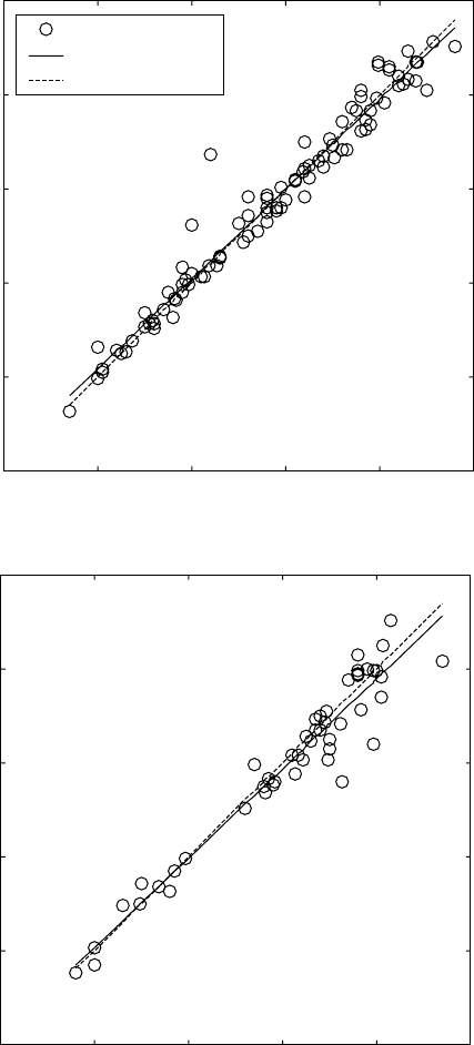
Two parameters are used to evaluate the performance of ANN modelling,
mean error and error deviation as defined below:
Mean error
=
1
( – )
=1
n
AT
i
n
ii
Σ
[14.1]
Error deviation
= ( ( – ) – ( ( – )) ) ( – 1)
22
nAT AT nn
ii ii
ΣΣ
[14.2]
In the above equations, A
i
is the calculated result for the i
th
alloy, T
i
is the
corresponding experimental value and n is the number of alloys in the sample
set. When two models have similar mean errors, both of which are smaller
than the target error (10 °C in the present case), the one of smaller error
deviation is considered to be better. The second column in Table 14.2 is a
statistical analysis of the data sets used for different purposes. When the
whole database is divided into different data sets in ANN modelling, ideally
the data in each data set should be of the same distribution. The second
column indicates that the data distribution is similar for the different data
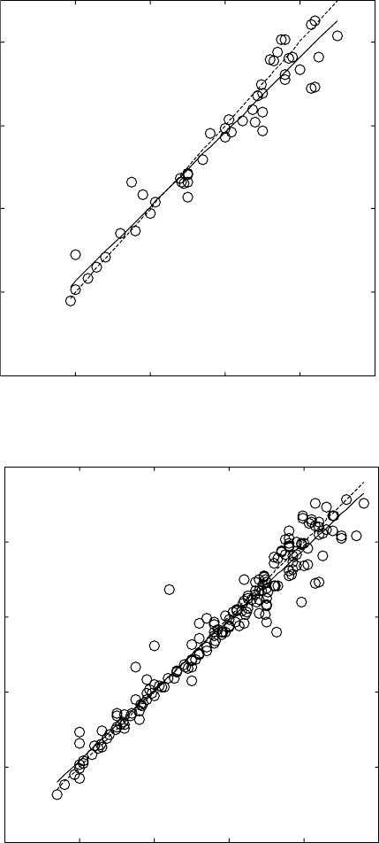
sets in this ANN model. Figure 14.2 illustrates the performance of this model
on different data sets. It can be seen that good model performance is achieved.
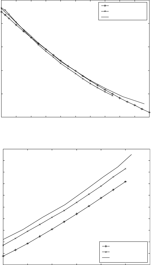
14.1.3 Phase diagram calculation of Ti–X systems
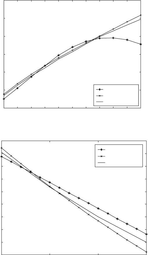
The influences of aluminium, molybdenum, vanadium, and oxygen on β
tr
temperature are quantified using the trained model. The experimental data
from literature and thermodynamic calculation using Thermo-Calc (Guo and
Sha, 2000) are also plotted for comparison (Figs. 14.3–14.6). The ANN
Table 14.2
Statistical analysis of ANN model (β-transus in °C)
Dataset Experimental Mean (
A
-
T
)* Standard
data deviation (
A
-
T
)*
Training data 883 ± 104 0 20
Validation data 907 ± 94 –7 24
Testing data 894 ± 100 –8 25
Whole dataset 892 ± 100 –4 23
*
A
: predicted results;
T
: experimental results
Neural network models and applications 337
Best linear fit: A = (0.959) T + (36.3)
Data points
Best linear fit
A = T
R = 0.982
600 700 800 900 1000 1100
T
(°C)
(a)
A (°C)
1100
1000
900
800
700
600
Best linear fit: A = (0.953) T + (35.6)
R = 0.966
600 700 800 900 1000 1100
T
(°C)
(b)
A (°C)
1100
1000
900
800
700
600
14.2
Performance of the neural network model of β-transus
temperature on: (a) training, (b) validation, (c) testing, and (d) whole
datasets.
Titanium alloys: modelling of microstructure338
Best linear fit: A = (0.895) T + (86.3)
R = 0.968
600 700 800 900 1000 1100
T
(°C)
(c)
A (°C)
1000
900
800
700
600
Best linear fit: A = (0.939) T + (50.4)
R = 0.974
600 700 800 900 1000 1100
T
(°C)
(d)
A (°C)
1100
1000
900
800
700
600
14.2
Contined
Neural network models and applications 339
model agrees with the experimental data very well. The error increases when
the element content is out of its compositional limit. For the Ti–Al system,
the error becomes very large when the amount of aluminium is over 7 wt.%.
In practice, the amount of aluminium in titanium alloys is usually limited to
β
tr
(°C)
1150
1100
1050
1000
950
900
850
ANN model
Thermo-Calc
Experimental
0123456 78 910
Al (wt.%)
14.3
β-transus of Ti-
x
Al alloy.
β
tr
(°C)
900
880
860
840
820
800
780
760
740
720
ANN model
Thermo-Calc
Experimental
0 5 10 15
Mo (wt.%)
14.4
β-transus of Ti-
x
Mo alloy.
Titanium alloys: modelling of microstructure340
7%, and the available data for higher aluminium amount is sparse. This is
thought to be the main reason for the large divergence at high aluminium
content.
Generally speaking, for Ti–X (X = Al, Mo, V, O) binary phase diagrams
β
tr
(°C)
900
850
800
750
700
650
New ANN model
Thermo-Calc
Experimental
0 2 4 6 8 10 12 14 16 18 20
V (wt.%)
14.5
β-transus of Ti-
x
V alloy.
β
tr
(°C)
960
950
940
930
920
910
900
890
880
870
860
New ANN model
Thermo-Calc
Experimental
0 0.1 0.2 0.3 0.4 0.5 0.6
O (wt.%)
14.6
β-transus of Ti-
x
O alloy.
