Sha W., Malinov S. Titanium Alloys: Modelling of Microstructure, Properties and Applications
Подождите немного. Документ загружается.

Neural network method 311
Training parameters
The next block in the computer program is for creating the neural network,
defining the training parameters and the actual training of the model. The
following matters are important in the design and training of neural networks:
(i) database and its distribution, (ii) choice of architecture of the neural
network, (iii) training algorithm and parameters, and (iv) transfer function.
Other training parameters, such as learning rate, performance goal, and
minimum performance gradient, may have a minor influence, but they aim
mainly at the optimisation of the training time and computer memory use,
and have little influence on the final performance of the trained model.
In the software developed on a user level, an option can be incorporated
to enable users to add their own data and re-train the model. This option will
be discussed in Section 13.4.1. Here, some recommendations on the selection
of the important parameters and their influences on the neural network
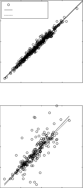
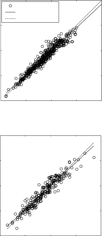
performance will be discussed. The reliability of the neural network model
for any particular combination of database distribution, architecture, training
algorithm and transfer function can be tested by an analysis of the network
response in a form of linear regression between network outputs (predictions)
and corresponding targets (experimental data) for the training and the testing
datasets (Fig. 13.5).
Different random division of a database into training and testing subsets,
using the computer program procedure which has been described, can result
in significantly different model performance for the same other parameters
(architecture, training algorithm, transfer function). This difference can be
explained with the ranges of input data variation for the training and the
testing datasets. In some cases of random dividing, instances may happen
where the range of variation of the data for the training dataset is narrow as
compared to the range of variation of the test dataset. In these cases, most of
the data pairs in the test datasets are new encounters for the trained NN and
fall outside the range of variables for which the model has been trained. An
appropriately trained NN model can give reliable predictions for new instances
within the ranges it has been trained (interpolation), but appreciable errors
are possible for predictions outside these ranges (extrapolation). Hence, it is
recommended that not only one but a number of training sessions with the
same other parameters but different random redistribution is carried out in
order to find the case with the most suitable dividing of the data to training
and testing sets.
The term ‘architecture of the neural network’ refers to the number of
layers in the NN and the number of neurons in each layer. The numbers of
neurons in the input layer and the output layer are determined by the numbers
of input and output parameters, respectively, while the number(s) of neurons
in the hidden layer(s) can vary. The number of the hidden layers could be
Titanium alloys: modelling of microstructure312
Train, Levenberg–Marquardt, 14 neurons
R = 0.989
Data points
Best linear fit
A = T
0 500 1000 1500 2000
Experimental yield strength (MPa)
(a)
Neural network predictions (MPa)
2000
1500
1000
500
0
Test, Levenberg–Marquardt, 14 neurons
R = 0.512
0 500 1000 1500 2000
Experimental yield strength (MPa)
(b)
Neural network predictions (MPa)
2000
1500
1000
500
0
13.5
Post-training linear regression analysis between experimental
data (
T
) and neural network predictions (
A
) for training (a,c) and
testing (b,d) datasets using Levenberg–Marquardt training without
(a,b) and with (c,d) Bayesian regularisation.
one, two or more. One hidden layer is enough for appropriate model
performance. Increasing the layers to two results in a remarkable increase of
the unknown parameters (connections) to be fitted, which itself increases
drastically the requirements for the amount of data without any noticeable
Neural network method 313
improvement in the final model performance (Malinov et al., 2001a). Hence,
in all the models discussed in this book (Figs 13.1 and 13.2), the general
structure of input, one hidden and one output layer, is used. In order to find
the optimal architecture, different numbers of neurons in the hidden layer
Train, Levenberg–Marquardt with Bayesian
regularisation, 14 neurons
R = 0.969
Data points
Best linear fit
A = T
0 500 1000 1500 2000
Experimental yield strength (MPa)
(c)
Neural network predictions (MPa)
2000
1500
1000
500
0
Test, Levenberg–Marquardt with Bayesian
regularisation, 14 neurons
R = 0.954
0 500 1000 1500 2000
Experimental yield strength (MPa)
(d)
Neural network predictions (MPa)
2000
1500
1000
500
0
13.5
Continued
Titanium alloys: modelling of microstructure314
should be tried. The number of neurons in the hidden layer (NNHL) influences
considerably the model performance. In what follows, some practical
recommendations for selection of NNHL by the user when re-training the
model with their own data are given. Two factors are important for determining
the number of neurons.
• First, the increase of the NNHL increases the connections and weights to
be fitted. The NNHL cannot be increased without limit because one may
reach a case where the number of the connections to be fitted is higher
than the number of the data pairs available for training. Though the
neural network can still be trained in this case, it is mathematically
undetermined and should be avoided. The maximum NNHL is different
for each particular case and depends on the number of inputs, number of
outputs and number of available data pairs. The number of the connections
to be fitted can be worked out by drawing the scheme of the NN (Fig.
13.3) for the particular case of inputs, outputs and NNH, and calculating
the connections to be fitted (Sha and Edwards, 2007).
• Second, the initial increase of the NNHL usually results in an improvement
of the model performance. However, one problem that can occur when
training with a large number of neurons is that the network can overfit
on the training set and not generalise well to new data. In other words,
the network is too flexible and the error of the training set is driven to
very small values, but when new data are presented to the network, the
error is large. The optimal NNHL depends on the database, nature of the
problem to be modelled and the training algorithm, and should be
determined for each particular case. The overfitting can be prevented by
different techniques aiming at better generalisation of the model.
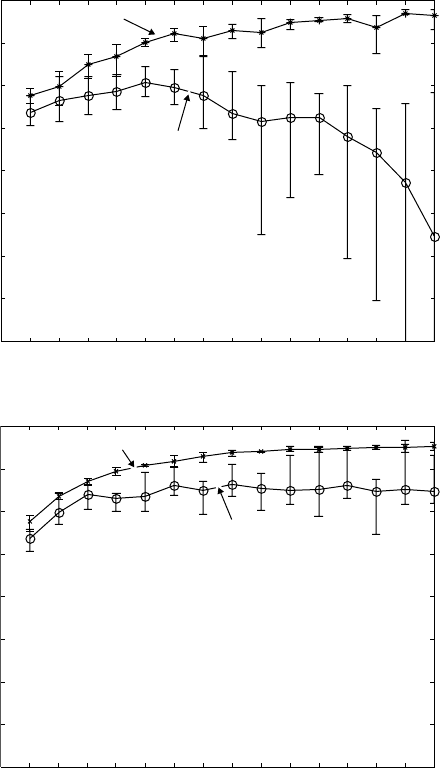
Figure 13.6 demonstrates one example of finding the optimal architecture of
the NN in terms of number of neurons in the hidden layer. The case is for the
prediction of yield strength of titanium alloys (Fig. 13.1b). The number of
inputs is 13, the number of outputs is 1 (if just yield strength is considered)
and the number of the available data pairs is 662 (441 for training and 221
for testing). In order to find the optimal architecture, different numbers of
neurons in the hidden layer were tried. The Levenberg–Marquardt training
algorithm was used for this study. The results for the influence of number of
neurons in the hidden layer on the NN response are given in Figs. 13.5 and
13.6. The results in Fig. 13.5 are for single training with 14 neurons in the
hidden layer and show the network response in a form of linear regression
analysis between the network outputs (predictions) and the corresponding
targets (experimental data), for two different training algorithms. The results
in Fig. 13.6 are presented in the form of correlation coefficient (R) between
the neural network predictions and the experimental data for the training and
the testing datasets, for different numbers of neurons in the hidden layer. For
Neural network method 315
each case, the values for the R coefficient are averaged from five separate
training runs under the same conditions and using different random divisions
of the dataset. When the number of neurons in the hidden layer is increased
from 1 to 5, the R coefficient for both training and test datasets quickly
Train
Test
01 23456 789101112131415
Number of neurons in the hidden layer
(a)
Regression coefficient
1
0.95
0.9
0.85
0.8
0.75
0.7
0.65
0.6
Train
Test
0 1 2 3 4 5 6 7 8 9 10 11 12 13 14 15
Number of neurons in the hidden layer
(b)
Regression coefficient
1
0.95
0.9
0.85
0.8
0.75
0.7
0.65
0.6
13.6
Regression coefficients between the neural network predictions
and the experimental data for different numbers of neurons in the
hidden layer using Levenberg–Marquardt training (a) without and (b)
with Bayesian regularisation.
Titanium alloys: modelling of microstructure316
increases (see Fig. 13.6a). Further increase in the number of neurons results
in further increase of the R coefficient for the training dataset that is approaching
the value of 1 (Figs. 13.5 and 13.6). However, the regression coefficient for
the test dataset quickly decreases to average values of <0.8 with large error
bars (Figs. 13.5 and 13.6). This observation shows that there is an effect of
overfitting when the number of neurons is increased to six and above. One
way to prevent the overfitting is by applying Bayesian regularisation in
combination with the Levenberg–Marquardt training (Figs. 13.5 and 13.6).
This is one of the techniques aiming at better generalisation. The results
obtained for the different numbers of neurons in the hidden layer are appreciably
stable (see Fig. 13.6b). Values of coefficient R for both training and test
datasets increase when the number of the neurons is increased to eight.
Further increase of neurons does not result in overfitting and the results for
the regression analyses of both training and test datasets are comparable (see
Fig. 13.5c,d). However, at the same time, increasing the number of neurons
above eight does not give appreciable improvement, while the training time
is significantly increased. Considering all the above, the optimal for this
neural network architecture is eight neurons in the hidden layer.
The type of the training algorithm used is important for both neural network
response and central processing unit (CPU) time (or computational resources)
necessary for training. A summary analysis of the influence of different
training algorithms on the performance of the neural network model is given
below. Different training options can be carried out, including training on
variations of mean square error for better generalisation, training against a
validation set, and training until the gradient of the error reaches a minimum.
Improvement of the generalisation can be achieved by means of regularisation
and early stopping with validation. The general opinion is that automated
regularisation based on Bayesian regularisation in combination with
Levenberg–Marquardt training usually gives the best result, in terms of model
performance and training speed. This combination is used in the neural
networks described in this book unless otherwise stated. However, in some
cases, other training algorithms such as one-step-secant, Polak–Ribiere
conjugate gradient, and variable learning rate may give competitive results.
In the software developed and described in this book, the user can choose the
training algorithm to predict values or re-train the model.
The transfer function transforms the neuron input value into the output
value. The most popular functions are hard limit (hardlim), linear (purelin),
log sigmoid (logsig), and hyperbolic tangent sigmoid (tansig). For all cases
of NN, a linear transfer function is suitable in the output layer. The transfer
functions in the hidden layer are generally s-shaped curves, with the output
value confined within limits of (0,1) or (–1,1), for log-sigmoid and tan-
sigmoid functions, respectively. Mathematical formulations of the main transfer
functions and their general shapes can be found in Chapter 14. In the model
Neural network method 317
developed and described in this book, different transfer functions in the
hidden layers were attempted. Mainly, log sigmoid and tangent sigmoid
functions are compared. It may be concluded that there is little influence
whether log sigmoid and tangent sigmoid functions are used. Hence, this is
not considered as a significant parameter for the NN response. In all models
(Fig. 13.1), in their final version, hyperbolic tangent sigmoid function is
used for the neurons in the hidden layer.
Optimal model parameters
The computer program for the design of the neural network model is written
in a way to find the best combination of database distribution, network
architecture and training algorithm, by grid search (Fig. 13.4). Loops are
organised for the above parameters. By varying these, all possible combinations
of network architecture and training algorithm with different database
distributions are attempted and stored. For each combination, the correlation
coefficients between the neural network predictions and the experimental
data for the training and the testing datasets are stored and used for further
evaluation. The program realisation is as follows. First, the number of neurons
in the hidden layer is put equal to one, and the first training algorithm, for
example one-step-secant, is used. For this combination, at least five sessions
of training with different random redistributions of the database are executed.
Next, the number of the neurons is increased to two, and again five sessions
of training with different random redistributions (but the same as those for
the above case and for all cases) of the database are executed. The same is
executed for three, four, five, etc. number of neurons in the hidden layer. The
NNHL is increased as far as the case remains mathematically determined
(see above). The next loop is to change the training algorithm and the same
procedure is repeated for the new and for all the training algorithms given
above. In this way, we have stored neural networks trained with all possible
combinations of network architecture and training algorithm and different
random redistributions of the datasets. The next is to find the best case. To
do this, the following procedure is applied. First, using the runs with different
random redistributions, the average regression coefficients between neural
network predictions and the experimental data for the training and the testing
datasets, for different network architecture and training algorithms, are
calculated. For one training algorithm, the regression coefficients after training
with different NNHL are compared, and the best case (the winner), in terms
of best architecture for this training algorithm, is found. This procedure is
executed for each training algorithm. The winners for the different training
algorithms are thereafter compared and the best combination of network
architecture and training algorithm is found. For this combination, the best
case among the five sessions of training with different random redistributions
Titanium alloys: modelling of microstructure318
is extracted and this is the final winner in the sense of best database distribution,
network architecture and training algorithm. This case is then stored and the
neural network trained with these parameters is used for further simulations
and predictions. The above procedure is executed for all the models in Fig.
13.1, and the best cases are used with the corresponding graphical user
interface (GUI), in Fig. 13.2. Readers should be reminded that the optimal
combination of database distribution, network architecture and training
algorithm depends on many factors, such as the nature of the problem to be
modelled, the number of inputs and outputs, and the database available, and
can differ considerably from case to case. The computer program and the
procedure described above for finding the optimal case of trained neural
network, and reliable neural network modelling in general, require significant
amounts of data, but, once trained and created, the model can quickly and
easily be used to predict for new instances.
Post-training procedures
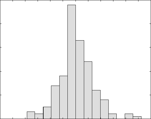
The next block of the computer program is for further experimental verification
of the model by statistical analysis of the error of the model predictions. The
relative error (relative difference between the model simulations and the
experimental data) is calculated for each data pair. The results are presented
by plotting them in the classical plot of occurrence versus error, also referred
to as frequency versus error. This plot is more informative as compared to
the plots of the linear regression analysis (Fig. 13.5). Using it, the specialists
in the field can conclude whether the achieved accuracy in terms of error
variation is acceptable for the phenomenon being modelled. Here, an example
is given of such an analysis for modelling of the modulus of elasticity of
titanium alloys (Fig. 13.7). Additional plots and analyses for other correlations
are given and discussed by Malinova et al. (2001a).
Further verification of the model simulations can be performed by the
user by means of direct comparison of the software predictions and experimental
data. Users can utilise the software and the GUIs developed (Fig. 13.2) to
calculate results for new input values and thereafter can compare these
predictions with experimental data taken from the literature or with their
own experimental data. This procedure is not part of the program and is
executed manually by the user. Some comparisons of this type are given by
in Malinova et al. (2001a).
In all the models in Figs. 13.1 and 13.2, very good performance is achieved.
Good agreement between the experimental and calculated values is found.
Neural network method 319
13.3 Use of the software
13.3.1 General organisation of the software and
graphical user interfaces
The software system should be designed in a modular fashion, with each
module designed in such a way that it can be upgraded by a later version
without substantially affecting the operation of the remainder of the model.
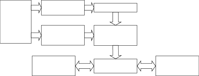
The different modules are linked according to the block diagram given in
Fig. 13.8. The modules for databases, computer program for training and
trained ANN are described in the previous section. Once the neural network
models are trained and verified, they can be used for further simulations and
predictions for arbitrary user defined new (unused in the training) combination
of input values, in order to reveal different correlations and phenomena in
titanium or during processing of titanium alloys. The interactions with the
system are organised by interface modules. For each of the models in Fig.
13.1, two types of interface are developed, namely text user interface and
graphical user interface (GUI). In the text version, the user is asked interactively
for input of the necessary information and, once it is completed, the output
from the system is generated.
On the basis of the designed models of artificial neural networks, graphical
user interfaces (Fig. 13.2) are developed using MatLab programming language
Min = – 7.81
Max = 10.42
Mean = 0.257
StDev = 2.963
–12 –10 –8 –6 –4 –20246 81012
Relative error ((E
exp
-E
calc
)/E
exp
) (%)
Occurrence
50
40
30
20
10
0
13.7
Post-training validation of the software simulations by statistical
analysis of the error of model simulations for modulus of elasticity.
Titanium alloys: modelling of microstructure320
Graphical
user
interfaces
for upgrade
of the
models
Module for new
data input
Module for input
of re-training
parameters
Module for
materials
selection
Databases
Computer
program for
training (learning)
Trained artificial
neural networks
Graphical user
interfaces for use
of the models
13.8
Block diagram of software system for modelling of correlations
in titanium alloys, based on artificial neural network approach.
that allows easy and further use of the models (Fig. 13.1). The user can run
any of the GUIs in Fig. 13.2 to input the desired new combination of input
values for each particular model using the textboxes, menus, list boxes, pop-
up menus, radio buttons, sliders, etc., provided (see Fig. 13.2). Once the
information is entered, the user can click on ‘Predict’ or ‘plot’. The information
entered is then acquired, organised and processed (see Fig. 13.8) as a new
input combination to the trained neural network for the corresponding GUI.
The trained artificial neural network calculates output for this combination
of inputs. The output is returned to the GUI, and is visualised in a form of
graph (in the cases in Fig. 13.1a,c) or dependence of the properties on a
desired parameter. In this way, the user can very easily obtain and evaluate
different kinds of dependence of any property involved in the models. In this
way, the user can easily obtain and evaluate the dependence of the outputs
from chosen input. Furthermore, the GUI provides an opportunity for easy
comparison of output properties corresponding to different sets of inputs,
by plotting them together. In the cases where the output is a graph, the
GUIs also allow smoothing of the predicted profile with a user-defined
coefficient.
The software system developed is based on trained artificial neural networks.
The training of the different modules is performed using the collected databases
for each particular case. However, the system is open for further upgrading
from the users, by adding additional data and training (see the left part of
Fig. 13.8). These features will be discussed in Section 13.4.1.
The block scheme given in Fig. 13.8 is for one of the models in Fig. 13.1
and the corresponding GUI in Fig. 13.2. In practice, in the software system
developed, all the GUIs in Fig. 13.2, as well as others, are integrated and
linked by an introductory GUI window. This allows easy switching between
the different applications. Such organisation is convenient for the user, because
once they have used any of the GUIs in Fig. 13.2 to predict a property (for
