Seminario J.M. Molecular and Nano Electronics. Analysis, Design and Simulation
Подождите немного. Документ загружается.


264 G. Stefanucci et al.
is the Slater determinant of the occupied eigenstates of the full, extended Hamiltonian
in equilibrium, H
s
t < 0. The practical question then arises as to how one can obtain
these eigenstates and how one can propagate them in time without having to deal
explicitly with the extended Hamiltonian. Below, we show how we have coped with
these problems.
4.1. Computation of KS eigenstates
Let us consider our electrode–junction–electrode system in equilibrium (t<0) and let
s
r =
Ej
r be the j-th degenerate eigenstate of energy E of the KS Hamiltonian H
s
.
The Green functions
RA
t t
and
<
t t
of the undisturbed system depend only on
the difference t −t
. In absence of magnetic fields, H
s
is invariant under time-reversal
and the imaginary part of the Fourier transformed
R
is simply given by
−
1
Im
rEr
=
E
E −E
d
E
j=1
E
j
r
∗
E
j
r
(66)
Multiplying Eq. (66) by
∗
Em
r
En
r
and integrating over r and r
in region C we
obtain
−
1
C
dr
C
dr
∗
Em
rIm
rEr
En
r
=
E
E −E
d
E
j=1
S
mj
E
S
jn
E
(67)
where
S
mj
E ≡
C
dr
∗
Em
r
Ej
r = S
∗
jm
E (68)
is the overlap matrix in region C between degenerate states. This matrix is Hermitian
and can be diagonalized, i.e.,
d
E
j=1
S
mj
Ea
l
j
E =
l
Ea
l
m
E (69)
Next, we multiply Eq. (67) by a
l
∗
m
Ea
l
n
E and sum over m and n. The result can be
written in terms of the new eigenfunctions a
El
r =
d
E
n=1
a
l
n
E
En
r as
−
1
C
dr
C
dr
a
∗
El
rIm
rEr
a
El
r
=
ll
2
l
E
E
E −E
(70)
where we have used Eq. (69) and the orthonormality of the S-matrix eigenvectors:
d
E
j=1
a
l
∗
j
Ea
l
j
E =
ll
. Equation (70) shows explicitly that the functions a
Ej
r
diagonalize Im
CC
E in the central region and that the eigenvalues are positive. Since
any linear combination of degenerate eigenstates is again an eigenstate, diagonalizing

Time-dependent transport phenomena 265
Im
CC
E gives us one set of linearly independent, degenerate eigenstates of energy
E. In our practical implementation described in more detail in Section 5, we diagonalize
−
1
D
C
E
Im
CC
E (71)
where D
C
E =−
1
Tr
Im
CC
E
is the total density of states in the central region.
If we use N
g
grid points to describe the central region, the diagonalization, in principle,
gives N
g
eigenvectors but only a few have the physical meaning of extended eigenstates
at this energy. It is, however, very easy to identify the physical states by looking at
the eigenvalues: at a given energy E only d
E
eigenvalues are nonvanishing and they
always add up to unity. The corresponding states are the physical ones. All the other
eigenvalues are zero (or numerically close to zero) and the corresponding states have
no physical meaning.
The procedure described above gives the correct extended eigenstates only up to
a normalization factor. When diagonalizing Eq. (71) with typical library routines one
obtains eigenvectors which are normalized to the central region. Physically this might
be incorrect. It is possible to fix the normalization by matching the wavefunction for
the central region to the known form (and normalization) of the wavefunction in the
macroscopic leads.
It should be emphasized that the procedure described here for the extraction of
eigenstates of the extended system from
CC
E only works in practice if E is in the
continuous part of the spectrum due to the sharp peak of the delta function in the discrete
part of the spectrum. Eigenstates in the discrete part of the spectrum can be found by
considering the original Schrödinger equation for the full system: H
s
= E. Using
again the block structure of the Hamiltonian this can be transformed into an effective
Schrödinger equation for an energy-dependent Hamiltonian for the central region only:
H
CC
+
=LR
H
C
1
E1
−H
H
C
C
=E
C
(72)
This equation has solutions only for certain values of E which are the discrete
eigenenergies of the full Hamiltonian H
s
. Since the left and right electrodes form a
continuum, the dimension of the kernel of E −H
is zero for those energies E in
the discrete part of the spectrum. We also notice that the second term in parenthesis in
Eq. (72) is nothing but the real part of the retarded/advanced self-energy in equilibrium,
see Eq. (47). Bound states as well as fully reflected waves will contribute to the density
but not to the current and might play a role in the description of charge-accumulation
in molecular transport, as, e.g., in Coulomb blockade phenomenon. In our TDDFT
formulation, bound states and fully reflected waves also play an extra role, since they
are needed for calculating the effective potential v
s
(which is a functional of the density)
which is in turn used for extracting all extended states.
4.2. Algorithm for the time evolution
In order to calculate the longitudinal current in an electrode–junction–electrode system
we need to propagate the KS orbitals. The main difficulty stems from the macroscopic

266 G. Stefanucci et al.
size of the electrodes whose remote parts, ultimately, are taken infinitely far away from
the central, explicitly treated, scattering region C.
The problem can be solved by imposing transparent boundary conditions [28] at the
electrode–junction interfaces. Efficient algorithms have been proposed for wave-packets
initially localized in the scattering region and for Hamiltonians constant in time. In this
section we describe an algorithm well suited for delocalized initial states, as well as for
localized ones, evolving with a time-dependent Hamiltonian.
Let H
s
t be the time-dependent KS Hamiltonian. We partition H
s
t as in Section 3.2.
The explicitly treated region C includes the first few atomic layers of the left and right
electrodes. The boundaries of this region are chosen in such a way that the density
outside C is accurately described by an equilibrium bulk density. It is convenient to
write H
t, with =L R, as the sum of a term H
0
=H
0 which is constant in
time and another term U
t which is explicitly time-dependent, H
t =H
0
+U
t.
In configuration space, U
t is diagonal at any time t since the KS potential is local
in space. Furthermore, the diagonal elements U
rt are spatially constant for metallic
electrodes. Thus, U
t =U
t1
and U
L
t −U
R
t is the total potential drop across
the central region. We write H
s
t =
˜
Ht +U t with
˜
Ht =
⎡
⎣
H
0
LL
H
LC
0
H
CL
H
CC
t H
CR
0 H
RC
H
0
RR
⎤
⎦
and U t =
⎡
⎣
U
L
t1
L
00
000
00U
R
t1
R
⎤
⎦
(73)
In this way, the only term in
˜
Ht that depends on t is H
CC
t. For any given initial
state 0=
0
we calculate t
m
=mt=
m
by using a generalized form
of the Cayley method
1+i
˜
H
m
1+i
2
U
m
1−i
2
U
m
m+1
=
1−i
˜
H
m
1−i
2
U
m
1+i
2
U
m
m
(74)
with
˜
H
m
=
1
2
˜
Ht
m+1
+
˜
Ht
m
, U
m
=
1
2
Ut
m+1
+Ut
m
and = t/2. It should
be noted that our propagator is norm conserving (unitary) and accurate to second order
in , as is the Cayley propagator [29]. Denoting by
the projected wave function
onto the region = R L C, we find from Eq. (74)
m+1
C
=
1
C
−iH
m
eff
1
C
+iH
m
eff
m
C
+S
m
−M
m
(75)
Here, H
m
eff
is the effective Hamiltonian of the central region:
H
m
eff
=H
m
CC
−iH
CL
1
1
L
+iH
0
LL
H
LC
−iH
CR
1
1
R
+iH
0
RR
H
RC
(76)
with H
m
CC
=
1
2
H
CC
t
m+1
+H
CC
t
m
. The source term S
m
describes the injection
of density into the region C, while the memory term M
m
is responsible for the
hopping in and out of the region C. In terms of the propagator for the uncontacted and
undisturbed electrode
g
=
1
−iH
0
1
+iH
0
(77)
Time-dependent transport phenomena 267
the source term can be written as
S
m
=−
2i
1
C
+iH
m
eff
=LR
!
m0
u
m
H
C
g
m
1
+iH
s
0
(78)
with
u
m
=
1−i
2
U
m
1+i
2
U
m
and !
mk
=
m
!
j=k
u
j
2
(79)
For a wave packet initially localized in C the projection onto the left and right
electrode
0
vanishes and S
m
=0 for any m, as it should be. The memory term
is more complicated and reads
M
m
=−
2
1
C
+iH
m
eff
=LR
m−1
k=0
!
mk
u
m
u
k
Q
m−k
+Q
m−k−1
×
k+1
C
+
k
C
(80)
where
Q
m
=H
C
g
m
1
+iH
s
H
C
(81)
The quantities Q
m
depend on the geometry of the system and are independent of the
initial state
0
.
Below, we propose a recursive scheme to calculate the Q
m
’s for those system
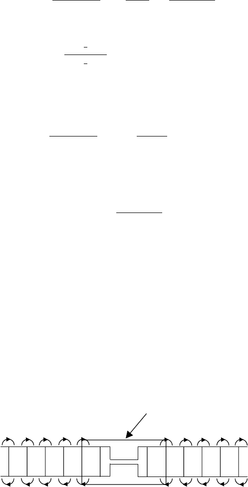
geometries having semiperiodic electrodes along the longitudinal direction, see Figure 3.
In this case H
0
has a tridiagonal block form
H
0
=
⎡
⎢
⎢
⎣
h
V
0
V
h
V
0 V
h
⎤
⎥
⎥
⎦
(82)
where h
describes a convenient cell and V
is the hopping Hamiltonian between two
nearest neighbor cells. Without loss of generality we assume that both h
and V
Region C
....
V
L
h
L
h
L
h
L
h
L
h
L
h
R
h
R
h
R
h
R
h
R
V
L
V
L
V
L
V
L
V
R
V
R
V
R
V
R
V
R
V
R
V
R
V
R
V
R
V
R
V
L
V
L
V
L
V
L
V
L
....
Figure 3 Schematic sketch of an electrode–junction–electrode system with semiperiodic
electrodes.

268 G. Stefanucci et al.
are square matrices of dimension N
×N
. Taking into account that the central region
contains the first few cells of the left and right electrodes, the matrix Q
m
has the
following structure
Q
m
L
=
⎡
⎣
q
m
L
00
000
000
⎤
⎦
Q
m
R
=
⎡
⎣
00 0
00 0
00q
m
R
⎤
⎦
(83)
The q
m
’s are square matrices of dimension N
×N
and are given by
q
m
=V
g
m
1
+iH
$
11
V
(84)
where the subscript 1 1 denotes the first diagonal block of the matrix in the square
brackets. We introduce the generating matrix function
q
x y ≡ V
1
x1
+iyH
$
11
V
(85)
which can also be expressed in terms of continued matrix fractions
q
x y = V
1
x +iyh
+y
2
2
V
1
x +iyh
+y
2
2
V
1
V
V
V
=V
1
x +iyh
+y
2
2
q
x y
V
(86)
The q
m
’s can be obtained from
q
m
=
1
m!
−
x
+
y
$
m
q
x y
%
%
%
%
x=y=1
(87)
From Eqs (87) and (86) one can build up a recursive scheme. Let us define
p
−1
x y = x +iyh
+y
2
2
q
x y
and
p
m
=
1
m!
−
x
+
y
$
m
p
x y
%
%
%
%
x=y=1
Then, by definition, q
m
=V
p
m
V
. Using the identity
1
m!
−
x
+
y
$
m
p
x yp
−1
x y = 0
one finds
1+ih
p
m
=1 −ih
p
m−1
−
2
m
k=0
q
k
+2q
k−1
+q
k−2
p
m−k
(88)

Time-dependent transport phenomena 269
with p
m
= q
m
= 0 for m<0. Once q
0
has been obtained by solving Eq. (86) with
x =y =1, we can calculate p
0
=1+ih
+
2
q
0
−1
. Afterwards, we can use Eq. (88)
with q
1
=V
p
1
V
to calculate p
1
and hence q
1
and so on and so forth.
This concludes the description of our algorithm for the propagation of the time-
dependent Schrödinger equation for extended systems. It is worth mentioning an
additional complication here which arises for the propagation of a time-dependent Kohn–
Sham equation. This complication stems from the fact that in order to compute
m+1
C
at time step m +1, one needs to know the time-dependent KS potential at the same
time step which, via the Hartree and exchange-correlation potentials, depends on the
yet unknown orbitals
m+1
C
. Of course, the solution is to use a predictor-corrector
approach: in the first step one approximates H
m
CC
by H
CC
t
m
, computes new orbitals
˜
m+1
C
and from those obtains an improved approximation for H
m
CC
.
5. Implementation details for one-dimensional systems
and numerical results
All the methodological discussion of Section 4 is general and can be applied to all
systems having a longitudinal geometry like the one in Figure 3. In this section we show
that the proposed scheme is feasible by testing it against one-dimensional model systems.
The extension to real molecular-device configurations is presently under development
[30]. We consider systems described by the Hamiltonian
xHx
=x −x
−
1
2
d
dx
2
+Vx
$
(89)
We have used a simple three-point discretization for the second derivative
d
2
dx
2
x
x=x
i
≈
1
x
2
x
i+1
−2x
i
+x
i−1
(90)
with equidistant grid points x
i
, i =1N
g
and spacing x. Within this approximation,
matrices of the form H
C
MH
C
, which are N
g
×N
g
matrices and appear, e.g., in Eq. (38)
or (81), have only one nonvanishing matrix element. For =L this is the 1 1 element,
for = RitistheN
g
N
g
element.
In order to proceed, we have to specify the nature of the leads and therefore the
lead Green function. Here we choose the simplest case of semi-infinite, uniform leads
at constant potential U
0
. In this case, the retarded Green function g
R
in the energy
domain can be given in closed form:
g
R
E
kl
=−
ix
&
2
˜
E
exp
'
i
&
2
˜
E
x
k
−x
l
(
+
ix
&
2
˜
E
exp
'
i
&
2
˜
E
x
k
−x
0
+x
l
−x
0
(
(91)
with
˜
E
= E −U
0
. The abscissa x
0
is the position of the interface between the lead
and the device region; in our implementation x
L0
is the first grid point of region C
270 G. Stefanucci et al.
while x
R0
is the N
g
-th grid point of region C. According to the notation in Eq. (63)
the one-particle state of region C describing an electron localized in x
L0
is denoted by
x
C1
while the one-particle state of region C describing an electron localized in x
R0
is
denoted by x
CN
g
. The coordinate x
k
= x
0
±kx, k>0, where the plus sign applies
for = R and the minus sign for = L.
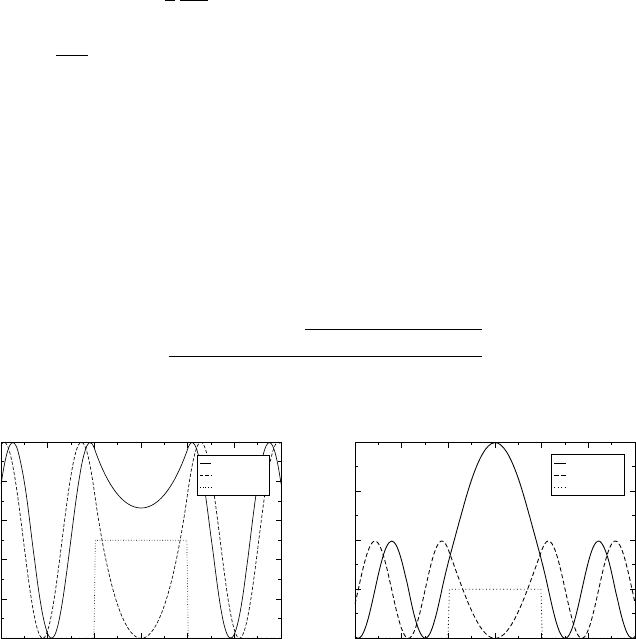
The results of the procedure for calculating extended eigenstates as described in
Section 4.1 are illustrated in Figure 4 for a square potential barrier with zero potential
in both leads. In the left panel we have the square modulus of eigenstates at an energy
below the barrier height, while in the right panel eigenstates with energy higher than the
barrier are shown. The states result from diagonalization of Eq. (71). In order to obtain
the normalization constant we compute the logarithmic derivative at the boundary of
the central region numerically and match it to the analytic form in the lead to obtain the
phase shift
:
1
2
d
2
dx
2
lnx
2
%
%
%
%
x=x
0
=q cot
(92)
where q =
&
2
˜
E
. Knowing the phase shift we can rescale the wavefunction such that it
matches with the analytic form sinqx −x
0
+
at the interface. Of course, this form
of the extended states only applies for
˜
E
> 0 but as long as E is in the continuous part
of the spectrum, it is correct at least for one of the leads. This is sufficient to determine
the normalization. The states obtained numerically with this procedure coincide with
the known analytical results.
We then implemented the propagation scheme presented in the previous section.
Within our three-point approximation, h
, V
and q
are 1 ×1 matrices. The equation
for q
0
[see Eqs (86) and (87)] becomes a simple quadratic equation which can be
solved explicitly
q
0
=
−1+ih
+
)
1+ih
2
+4V
2
2
2
(93)
–6 –4 –2
x /au x /au
0
0.2
0.4
0.6
0.8
1
|ψ (x)|
2
|ψ (x)|
2
V(x)/au
V(x)/au
gerade
ungerade
potential
0
0.5
1
1.5
2
gerade
ungerade
potential
6420–6–4–26420
Figure 4 Continuum states of square potential barrier at different energies with leads at zero
potential. Left panel: eigenstates for = 045au, just below the barrier height of 0.5 au. Right
panel: eigenstates at = 06au
Time-dependent transport phenomena 271
Although the quadratic equation has two solutions, the above choice for q
0
is dictated
by the fact that the Taylor expansions for small of Eqs (93) and (86) have to coincide.
Using this result we then solved the iterative scheme to obtain the q
m
for m ≥ 1.
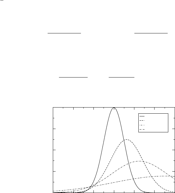
As a first check on the propagation method we propagated a Gaussian wavepacket
which, at initial time t = 0, is completely localized in the central device region. (The
source terms S
m
then vanish identically.) As can be seen in Figure 5, the wavepacket
correctly propagates through the boundaries without any spurious reflections.
For the propagation of the extended initial states (the eigenstates of the unper-
turbed system) we also need to implement the source terms S
m
. In the follow-
ing we assume that the left and right leads are at the same potential initially so
that the analytic form of the initial states is in both leads given by sinqx −x
0
+
=
expi
−iqx
0
expiqx −cc
/2i. Let us specialize the discussion to the
case = R and define the state q
R
according to x
Rk
q
R
=expiqkx, where
x
Rk
is the one-particle state of electrode R describing an electron localized in x
k
=
x
R0
+kx, k>0. Then, the projection of the initial state onto lead R reads
0
R
=
1
2i
expi
q
R
−exp−i
−q
R
. From Eq. (78) the contribution to the source term
for = R is completely known once we know how H
CR
g
R
m
/1
R
+iH
RR
acts on
the state q
R
. We have
H
CR
g
R
m
1
R
+iH
RR
q
R
=V
R
x
CN
g
x
R1
g
R
m
1
R
+iH
RR
q
R
(94)
where x
CN
g
corresponds the N
g
-th discretization point of region C (the last point on the
right before electrode R starts). We rewrite the unknown quantity as follows
*
x
R1
%
%
%
%
g
R
m
1
R
+iH
RR
%
%
%
%
q
R
+
=
Dx y
m
m!
"x y
%
%
%
%
x=y=1
(95)
–6–4–20246
x /au
0
0.1
0.2
0.3
0.4
|ψ(x)|
2
t = 0.0 au
t = 2.5 au
t = 5.0 au
t = 10 au
Figure 5 Time evolution of a Gaussian wavepacket with initial width 1.0 au and initial
momentum 0.5 au for various propagation times. The transparent boundary conditions allow the
wavepacket to pass the propagation region without spurious reflections at the boundaries

272 G. Stefanucci et al.
with
Dx y =
,
−
x
+
y
-
"x y =x
R1
1
x1
R
+iyH
RR
q
R
(96)
Next, we use the Dyson equation to find an explicit expression for "x y. We have
1
x1
R
+iyH
RR
q
R
=
1
x
q
R
−
1
x
iy
x1
R
+iyH
RR
H
RR
q
R
(97)
It is straightforward to realize that the action of H
RR
on q
R
yields
H
RR
q
R
=2V
R
cosqx +h
R
q
R
−V
R
e
−iqx
x
R1
(98)
so that Eq. (97) can be rewritten as
1+
2iyV
R
cosqx
x
$
1
x1
R
+iyH
RR
q
R
=
1
x
q
R
+
1
x
iyV
R
e
−iqx
x1
R
+iyH
RR
x
R1
(99)
Projecting Eq. (99) on x
R0
we find
1+
2iyV
R
cosqx
x
$
"x y =
1
x
+
iye
−iqx
xV
R
q
R
x y (100)
where q
R
x y is the generating function defined in Eq. (85). Solving Eq. (100) for
"x y we conclude that
V
R
"x y =
V
R
+iye
−iqx
q
R
x y
x +2iyV
R
cosqx +h
R
(101)
Using the relation in Eq. (87) for the coefficients q
m
we find
Dx y
m
m!
"x y
%
%
%
%
x=y=1
=
1−2iV
R
cosqx +ih
R
m
1+2iV
R
cosqx +ih
R
m+1
+
i
V
R
e
−iqx
×
m
j=0
1−2iV
R
cosqx +ih
R
m−j
1+2iV
R
cosqx +ih
R
m+1−j
q
j
R
+q
j−1
R
(102)
One may proceed along the same lines for extracting the left component of the
source term.
To test our implementation we have propagated eigenstates of the extended system.
As expected, these states just pick up an exponential phase factor exp−iEt during the
propagation.
We are now in a position to apply our algorithm to the calculation of time-dependent
currents in one-dimensional model systems. The systems are initially in thermodynamic
equilibrium. At time t = 0, a time-dependent perturbation is switched on. In all the
examples below the current is calculated according to Eq. (62):
Ix t = 2
k
F
−k
F
dk
2
Im
,
∗
k
x t
d
dx
k
x t
-
=2
k
F
0
dk
2
Im
,
∗
k
d
dx
k
+
∗
−k
d
dx
−k
-
(103)
Time-dependent transport phenomena 273
where the prefactor 2 comes from spin and k
F
=
)
2
F
is the Fermi wavevector of a
system with Fermi energy
F
.
5.1. DC bias
As a first example we considered a system where the electrostatic potential vanishes
identically both in the left and right leads as well as in the central region which is
explicitly propagated. Initially, all single particle levels are occupied up to the Fermi
energy
F
.Att = 0 a constant bias is switched on in the leads and the time-evolution
of the system is calculated. We chose the bias in the right lead as the negative of the
bias in the left lead, U
R
=−U
L
.
The numerical parameters are as follows: the Fermi energy is
F
=03 au, the bias is
U
L
=−U
R
=005 0 15 025au, the central region extends from x =−6tox =+6au
with equidistant grid points with spacing x = 003 au. The k-integral in Eq. (103) is
discretized with 100 k-points, which amounts to a propagation of 200 states. The time
step for the propagation was t = 10
−2
au.
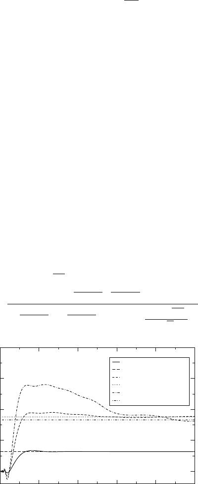
In Figure 6 we have plotted the current densities at x = 0 as a function of time for
different values of the applied bias. As a first feature we notice that a steady state is
achieved, in agreement with the discussion of Section 3.3. The corresponding steady-
state current I
S
can be calculated from the Landauer formula. For the present geometry
this leads to the steady current
I
S
= 8e
maxU
L
U
R
d
2
f −U
L
−f −U
R
×
√
−U
L
√
−U
R
√
−U
L
+
√
−U
R
2
+U
L
U
R
sinl
√
2
√
$
2
(104)
20080100
t /au
0
0.05
0.1
0.15
0.2
I /au
U = 0.05
U = 0.05 steady state
U = 0.15
U = 0.15 steady state
U = 0.25
U = 0.25 steady state
6040
Figure 6 Time evolution of the current for a system where initially the potential is zero in the
leads and the propagation region. At t = 0, a constant bias with opposite sign in the left and
the right leads is switched on, U = U
L
=−U
R
(values in atomic units). The propagation region
extends from x =−6tox =+6au. The Fermi energy of the initial state is
F
= 03au. The
current in the center of the propagation region is shown