Seminario J.M. Molecular and Nano Electronics. Analysis, Design and Simulation
Подождите немного. Документ загружается.


244 M. Tsukada et al.
6. Carrier transport process
In this section, the carrier transport in the molecular bridge is discussed in the model of
the previous section. Here the states of the electrodes are expressed as
m
L
left
=
0
m
L
(for left electrode) (17a)
m
R
right
=
N +1
m
R
(for right electrode) (17b)
Transition rates from a state “a” to another state “b” is calculated by Fermi’s golden
rule as
W
a→b
=
2
h
m
b
H
ab
2
E
a
−E
b
m
a
(18)
The state “a” or “b” is defined in Eq. (15) or (17a) or (17b), and the matrix element
H
ab
and the energy E
a
are calculated by
E
a
=
m
a
a
H
total
m
a
a
(19)
H
ab
=
m
a
a
H
total
m
b
b
(20)
In Eq. (18),
m
a
means the thermal average with the vibration state of “a”. In the
following, temperature is set to 0 Kelvin.
The carrier transport can be analyzed from the population probability
P
a
t
obtained
by the master equation,
dP
a
t
dt
=
b
W
b→a
P
b
t −
b
W
a→b
P
a
t (21)
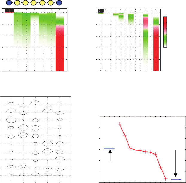
Figures 12(a) and (b) shows the time-dependent occupation of each site and state,
respectively. The 0th and 6th sites in Figure 12(a) means the left or right electrode.
Before t = 0 the carrier is assumed to be in the left electrode. At t = 0, we started
to solve the master equation of Eq. (12). In other words, the injection from the left
electrode to the molecular bridges started at t = 0. When time goes by, the occupation
at the left electrode rapidly decreases, and the occupation at the sites 1, 2, 4, 5 increases
as shown in Figure 12(a). After 0.1 fsec, the occupation of the 6th site at the right
electrode increases and finally becomes “1”.
The time-dependent occupation of each state is shown in Figure 12(b). At first, the 8th
state is occupied and then the 7th , 5th and 2nd states are occupied. After these processes,
the 0th state in right electrode is finally occupied. We analyze these processes by the
wavefunction and the energy levels. The wavefunctions in the molecular bridges are
shown in Figure 12(c). Notice that because a different value of the coupling parameter
is assumed ( =08, the composition of each state is somewhat different from the case
of Figure 11 ( =16. The energy level of each state from 0 through 11 in the electrodes
and the molecules are shown in Figure 12(d). From Figure 12(c) and (d), the 8th state
has a large amplitude at the 1st site, i.e., the site closest to the left electrode and its
Quantum electron transport for molecular devices 245
0
0.1
0.2
0.3
0.4
0.5
01234
5
6
Time (psec)
Site
(a)
0
0.2
0.1
0.3
0.4
0.5
Time (psec)
State
11
0123456789
Population
1
0.8
0.6
0.4
0.2
0
(b)
Right
electrode
Left
electrode
State
Energy (eV)
1
1.5
0.5
0
–0.5
–1
–1.5
1314 121110 9 8 7 6 5 4 3 2 1 0 –1–2
(d)
10
9
8
7
6
5
5
4
4
3
3
2
1
21
State
Site
(c)
10
Figure 12 Time-dependent occupation of each (a) site and (b) state, for the case with the state
components and the levels are shown in (c) and (d), respectively
energy is near the level of the left electrode. So it is easy to understand why the 8th
state becomes occupied at the earliest stage. By analyzing the relative magnitudes of
the transition rate W
i→k
, the most probable path is 11th (left) → 8th → 7th → 5th →
2nd→ 1st→ 0th (right). This is consistent with the result of Figure 12. The rate of W
2→1
has a smaller value and this is a rate-limiting step. The reasons for the small W
2→1
are:
first, the 2nd state has a node at the 3rd site while the 1st state does not have a node:
second, a large energy gap exists between the two states 1 and 2, which suppresses
the transition. The transition rates W
7→6
and W
5→4
are also negligibly small, because
of the almost orthogonal character between the states 6 and 7, or between the states 5
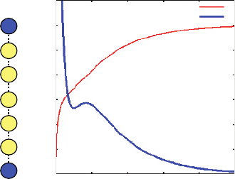
and 4. In Figure 13, the center of the charge and its velocity are shown as functions of
time. For bulk organic materials, time-of-flight (TOF) experiments are frequently used
to estimate the carrier mobility. The result of the velocity in Figure 13 is similar to that
observed by TOF. Therefore, this might indicate the method of the estimation for the
carrier mobility in the molecular bridges described above is legitimate.
246 M. Tsukada et al.
0
0
1
2
3
5
4
6
7
0.1 0.2 0.3 0.4 0.5
Time (psec)
X (center) (site)
Velocity (site/psec)
35
30
25
20
15
5
10
0
X (center)
Velocity
Figure 13 The time dependence of the center of mass position and the velocity of the carrier
References
[1] James M. Tour, Molecular Electronics, World Scientific, 2003.
[2] M. Tsukada, K. Tagami, K. Hirose and N. Kobayashi, J. Phys. Soc. Jpn., 74 (2005) 1079.
[3] J. Taylor, H. Guo and J. Wang, Phys. Rev. B 63 (2001) 245407.
[4] S. Datta, Electronic Transport in Mesoscopic System (Cambridge University Press, Cam-
bridge, U.K., 1995).
[5] K. Tagami and M. Tsukada, Curr. Appl. Phys. 3 (2003) 439.
[6] K. Tagami L. Wang and M. Tsukada, Nano Lett. 4 (2004) 209.
[7] K. Tagami and M. Tsukada, e-J.Surf. Sci. Nanotechnol. 2 (2004) 186.
[8] T. Frauenheim, G. Seifert, M. Elstner, T. Niehaus, C. Köhler, M. Amkreutz, M. Sternberg,
Z. Hajnal, A. D. Carlo and S. Suhai, J. Phys.: Condens. Matter, 14 (2002) 3015.
[9] K. Tagami and M. Tsukada, Jpn. J. Appl. Phys. 42 (2003) 3606.
[10] K. Tagami, M. Tsukada, Y. Wada, T. Iwasaki and H. Nishide, J. Chem. Phys. 119 (2003)
7491.
[11] K. Tagami and M. Tsukada, e-J. Surf. Sci. Nanotechinol. 1 (2003) 945.
[12] K. Tagami and M. Tsukada, e-J. Surf. Sci. Nanotechnol. 2 (2004) 205.
[13] K. Mitsutake and M. Tsukada, e-J. Surf. Sci. Nanotechnol. 4 (2006) 311.
Molecular and Nano Electronics: Analysis, Design and Simulation
J. M. Seminario (Editor)
© 2007 Elsevier B.V. All rights reserved.
Chapter 10
Time-dependent transport phenomena
G. Stefanucci
a
, S. Kurth
a
, E. K. U. Gross
a
and A. Rubio
b
a
Institut für Theoretische Physik, Freie Universität Berlin, Arnimallee 14, D-14195
Berlin, Germany and European Theoretical Spectroscopy Facility (ETSF)
b
Departamento de Física de Materiales, Facultad de Ciencias Químicas, UPV/EHU,
Unidad de Materiales Centro Mixto CSIC-UPV/EHU and Donostia International
Physics Center (DIPC), San Sebastián, Spain, and European Theoretical Spectroscopy
Facility (ETSF). hardy@physik.fu-berlin.de
1. Introduction
The aim of this chapter is to give a pedagogical introduction to our recently proposed
ab initio theory of quantum transport. It is not intended to be a general overview of
the field. For further information we refer the interested reader to [1–3]. The nomen-
clature quantum transport has been coined for the phenomenon of electron motion
through constrictions of transverse dimensions smaller than the electron wavelength,
e.g., quantum-point contacts, quantum wires, molecules, etc. The typical experimental
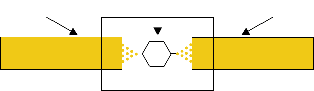
setup is displayed in Figure 1 where a central region C of meso- or nano-scopic size
is coupled to two metallic electrodes L and R which play the role of charge reservoirs.
The whole system is initially (at time t<0) in a well-defined equilibrium configuration,
described by a unique temperature and chemical potential (thermodynamic consistency).
The charge density of the electrodes is perfectly balanced and no current flows through
the junction.
As originally proposed by Cini [4], we may drive the system out of equilibrium by
exposing the electrons to an external time-dependent potential which is local in time and
space. For instance, we may switch on an electric field by putting the system between
two capacitor plates far away from the system boundaries. The dynamical formation
of dipole layers screens the potential drop along the electrodes and the total potential
turns out to be uniform in the left and right bulks. Accordingly, the potential drop is
entirely limited to the central region. As the system size increases, the remote parts
are less disturbed by the junction, and the density inside the electrodes approaches the
equilibrium bulk density.
247
248 G. Stefanucci et al.
Region C
Right electrode R
Left electrode L
t < 0
Figure 1 Schematic sketch of the experimental setup described in the text. A central region
which also includes few layers of the left and right electrodes is coupled to macroscopically large
metallic reservoirs. The system is in equilibrium for negative times
The Cini scheme can be combined with Time-Dependent Density Functional Theory
(TDDFT) [5]. In this theory, the time-dependent density of an interacting system moving
in an external, time-dependent local potential can be calculated via a fictitious system of
noninteracting electrons moving in a local, effective, time-dependent potential. Therefore
this theory is in principle well suited for the treatment of nonequilibrium transport
problems [6]. However, as far as the leads are treated as noninteracting, it is not obvious
that in the long time limit a steady-state current can ever develop. The reason behind
the uncertainty is that the bias represents a large perturbation and, in the absence of
dissipative effects, e.g., electron–electron or electron–phonon scattering, the return of
time-translational invariance is not granted. In this chapter we will show that the total
current tends to a steady-state value provided the effective potential of TDDFT is
independent of time and space in the left and right bulks. Also, the physical mechanism
leading to the dynamical formation of a steady state is clarified.
It should be mentioned that there has already been considerable activity in the density
functional theory (DFT) community to describe transport phenomena through systems
like the one in Figure 1. Most approaches are limited to the steady-state regime and
are based on a self-consistency procedure first proposed by Lang [7]. In this steady-
state approach based on DFT, exchange and correlation is approximated by the static
Kohn–Sham (KS) potential and the charge density is obtained self-consistently in the
presence of the steady current. However, the original justification involved subtle points
such as different Fermi levels deep inside the left and right electrodes (which is not
thermodynamically consistent) and the implicit reference of nonlocal perturbations such
as tunneling Hamiltonians within a DFT framework. (For a detailed discussion we refer
the reader to [8].) Furthermore, the transmission functions computed from static DFT
have resonances at the noninteracting KS excitation energies which in general do not
coincide with the true excitation energies.
Our TDDFT formulation, as opposed to the static DFT formulation, is thermody-
namically consistent, is not limited to the steady-state regime (we can study transients,
AC responses, etc.) and has the extra merit of accessing the true excitation energies of
interacting systems [9].
We will first use the nonequilibrium Green’s function (NEGF) technique to discuss
the implications of our approach. For those readers that are not familiar with the Keldysh

Time-dependent transport phenomena 249
formalism and with NEGF, in Section 2 we give an elementary introduction to the
Keldysh contour, the Keldysh–Green functions and the Keldysh book-keeping. The aim
of this section is to derive some of the identities needed for the discussion (thus providing
a self-contained presentation) and to establish the basic notation. In Section 3 we set up
the theoretical framework by combining TDDFT and NEGF. An exact expression for
the time-dependent total current It is written in terms of Green’s functions projected
in region C. It is also shown that a steady-state regime develops provided: (1) the KS
Hamiltonian globally converges to an asymptotic KS Hamiltonian when t →, (2) the
electrodes form a continuum of states (thermodynamic limit), and (3) the local density
of states is a smooth function in the central region. It is worth noting that the steady-state
current results from a pure dephasing mechanism in the fictitious KS system. Also, the
resulting steady current only depends on the KS potential at t =and not on its history.
However, the KS potential might depend on the history of the external applied potential
and the resulting steady-state current might be history dependent. A practical scheme to
calculate It is presented in Section 4. The main idea is to propagate the KS orbitals
in region C only, without dealing with the infinite and non-periodic system [10]. We
first show how to obtain the KS eigenstates
s
of the undisturbed system in Section 4.1.
Then, in Section 4.2 we describe an algorithm for propagating
s
under the influence
of a time-dependent disturbance. The numerical approach of Section 4 is completely
general and can be applied to any system having the geometry sketched in Figure 1. In
order to demonstrate the feasibility of the scheme we implement it for one-dimensional
model systems in Section 5. Here we study the dynamical current response of several
systems perturbed by DC and AC biases. We verify that for noninteracting electrons
the steady-state current does not depend on the history of the applied bias. Also, we
present preliminary results on net currents in unbiased systems as obtained by pumping
mechanisms. We summarize our findings and draw our conclusions in Section 6.
2. The Keldysh formalism
2.1. The Keldysh contour
In quantum mechanics we associate to any observable quantity O a hermitian operator
ˆ
O. The expectation
ˆ
O gives the value of O when the system is described by the
state . For an isolated system the Hamiltonian
ˆ
H
0
does not depend on time, and the
expectation value of any observable quantity is constant provided is an eigenstate
of
ˆ
H
0
. In this section we discuss how to describe systems which are not isolated but
perturbed by external fields. Without loss of generality, we assume that the system is
isolated for negative times t and that
ˆ
Ht < 0 =
ˆ
H
0
. The evolution of the state is
governed by the Schrödinger equation i
d
dt
t=
ˆ
Htt, and, correspondingly, the
value of O evolves in time as Ot =t
ˆ
Ot. The time-evolved state t=
ˆ
St 00, where the evolution operator
ˆ
St t
can be formally written as
ˆ
St t
=
T e
−i
t
t
d
¯
t
ˆ
H
¯
t
t>t
T e
−i
t
t
d
¯
t
ˆ
H
¯
t
t<t
(1)
In Eq. (1), T is the time-ordering operator and rearranges the operators in chronolog-
ical order with later times to the left;
T is the anti-chronological time-ordering operator.
250 G. Stefanucci et al.
The evolution operator is unitary and satisfies the group property
ˆ
St t
1
ˆ
St
1
t
=
ˆ
St t
for any t
1
. It follows that Ot is the average on the initial state 0 of the
operator
ˆ
O in the Heisenberg representation,
ˆ
O
H
t =
ˆ
S0 t
ˆ
O
ˆ
St 0, i.e.,
Ot =0
ˆ
S0 t
ˆ
O
ˆ
St 00
=0
Te
−i
0
t
d
¯
t
ˆ
H
¯
t
ˆ
OTe
−i
t
0
d
¯
t
ˆ
H
¯
t
0 (2)
We can now design an oriented contour with a forward branch going from t = 0
to t and a backward branch coming back from t and ending in t = 0, see Figure 2a.
Denoting with ¯z the variable running on , Eq. (2) can be formally recast as follows
Ot =0T
K
e
−i
d¯z
ˆ
H¯z
ˆ
Ot
0 (3)
The contour ordering operator T
K
moves the operators with “later” contour variable
to the left. A point z is later than a point z
if z
is closer to the starting point than
z, see Figure 2a. In Eq. (3),
ˆ
Ot is not the operator in the Heisenberg representation
[the latter is denoted with
ˆ
O
H
t]. Actually,
ˆ
Ot =
ˆ
O for any t. The reason for the
time argument stems from the need for specifying the position of the operator
ˆ
O in the
contour ordering.
Let us now extend the contour up to infinity, as shown in Figure 2b. For any physical
time t there are two points z =t
+
and z =t
−
on ; t
−
lies on the forward branch while
t
+
lies on the backward branch and it is later than t
−
according to the orientation cho-
sen. We have T
K
e
−i
d¯z
ˆ
H¯z
ˆ
Ot
−
=
ˆ
S0
ˆ
St
ˆ
Ot
ˆ
St 0 =
ˆ
S0 t
ˆ
O
ˆ
St 0 and
similarly T
K
e
−i
d¯z
ˆ
H¯z
ˆ
Ot
+
=
ˆ
S0 t
ˆ
Ot
ˆ
St
ˆ
S 0 =
ˆ
S0 t
ˆ
O
ˆ
St 0 Thus,
the expectation value Ot in Eq. (3) is also given by the formula
Oz =0T
K
e
−i
d¯z
ˆ
H¯z
ˆ
Oz
0 (4)
where is the contour in Figure 2b; is called the Keldysh contour [11, 12]. In
Eq. (4) the variable z can be either t
−
or t
+
and Ot
−
= Ot
+
= Ot.
The Keldysh contour can be further extended to account for statistical averages [13].
In statistical physics a system is described by the density matrix ˆ =
n
w
n
n
n
,
0
t
z ′
z
∞
t
t
–
+
t
(a)
(b)
–iβ
∞
0
–
0
–
(c)
γ
γ
γ
Figure 2 (a) The oriented contour described in the main text with a forward and a backward
branch between 0 and t. According to the orientation the point z is later than the point z
. (b) The
extended oriented contour described in the main text with a forward and a backward branch
between 0 and . For any physical time t we have two points t
±
on at the same distance from
the origin. (c) The generalization of the original Keldysh contour. A vertical track going from 0
to −i has been added and, according to the orientation chosen, any point lying on it is later than
a point lying on the forward or backward branch

Time-dependent transport phenomena 251
with w
n
being the probability of finding the system in the state
n
and
n
w
n
= 1.
The states
n
may not be orthogonal. We say that the system is in a pure state
if ˆ = . In a system described by a density matrix ˆ0 at t = 0, the time-
dependent value of the observable O is a generalization of Eq. (4), i.e., Oz =
n
w
n
n
0T
K
e
−i
d¯z
ˆ
H¯z
ˆ
Oz
n
0 Among all possible density matrices there is
one that is very common in physics and describes a system in thermal equilibrium:
ˆ = exp−
ˆ
H
0
−
ˆ
N/ with the inverse temperature , the chemical potential
, the operator
ˆ
N corresponding to the total number of particles and the grand-
partition function = Tr exp−
ˆ
H
0
−
ˆ
N. Assuming that
ˆ
H
0
and
ˆ
N commute, the
statistical average Oz with the thermal density matrix can be written as Oz =
Tr e
ˆ
N
e
−
ˆ
H
0
T
K
e
−i
d¯z
ˆ
H¯z
ˆ
Oz / We can now extend further the Keldysh contour
as shown in Figure 2c and define
ˆ
Hz =
ˆ
H
0
for any z on the vertical track. With this
definition
ˆ
Hz is continuous along the entire contour since
ˆ
H0 =
ˆ
H
0
. According to
the orientation displayed in the figure, any point lying on the vertical track is later than
a point lying on the forward or backward branch. We use this observation to rewrite
Oz as
Oz =
Tr
e
ˆ
N
T
K
e
−i
d¯z
ˆ
H¯z
ˆ
Oz
Tr
e
ˆ
N
T
K
e
−i
d¯z
ˆ
H¯z
(5)
where T
K
is now the ordering operator on the extended contour. It is worth noting
that the denominator in the above expression is simply . We have already shown that
choosing z on one of the two horizontal branches, Eq. (5) yields the time-dependent
statistical average of the observable O. On the other hand, if z lies on the vertical track
Oz =Tr e
ˆ
N
e
−i
−i
z
ˆ
H
0
ˆ
Oe
−i
z
0
ˆ
H
0
/ =Tr e
−
ˆ
H
0
−
ˆ
N
ˆ
O/ where the cyclic property
of the trace has been used. The result is independent of z and coincides with the thermal
average of the observable O.
To summarize, in Eq. (5) the variable z lies on the contour of Figure 2c; the r.h.s.
gives the time-dependent statistical average of the observable quantity O when z lies
on the forward or backward branch, and the statistical average before the system is
disturbed when z lies on the vertical track.
2.2. The Keldysh–Green function
The idea presented in the previous section can be used to define correlators of many
operators on the extended Keldysh contour. The Keldysh–Green function G is the
correlator of two field operators r and
†
r which obey the anticommutation
relations r
†
r
= r −r
. It is defined as
rGz z
r
=
1
i
Tr
e
ˆ
N
T
K
e
−i
d¯z
ˆ
H¯z
r z
†
r
z
Tr
e
ˆ
N
T
K
e
−i
d¯z
ˆ
H¯z
(6)
where the contour variable in the field operators specifies the position in the contour
ordering (there is no true dependence on z in and
†
). Here and in the following we

252 G. Stefanucci et al.
use boldface to indicate matrices in one-electron labels, e.g., G is a matrix and rGr
is the r r
matrix element of G. Due to the contour ordering operator T
K
, the Green
function G has the following structure
Gz z
= z z
G
>
z z
+z
zG
<
z z
(7)
where z z
=1ifz is later than z
on the contour and zero otherwise. We say that
a two-point function on the contour having the above structure belongs to the Keldysh
space. The Green function Gz z
obeys an important cyclic relation on the extended
Keldysh contour. As we shall see, the relations below play a crucial role since they
provide the boundary conditions for solving the Dyson equation. Choosing z = 0
−
we find
rG0
−
z
r
=−
1
i
Tr
e
ˆ
N
T
K
e
−i
d¯z
ˆ
H¯z
†
r
z
r
Tr
e
ˆ
N
T
K
e
−i
d¯z
ˆ
H¯z
(8)
where we have taken into account that 0
−
is the earliest time and therefore r 0
−
is
always moved to the right when acted upon by T
K
. The extra minus sign in the r.h.s.
comes from the contour ordering. More generally, rearranging the field operators and
†
(later arguments to the left), we also have to multiply by −1
P
, where P is the parity
of the permutation. Inside the trace we can move r to the left. Furthermore, we can
exchange the position of r and e
ˆ
N
by noting that re
ˆ
N
=e
ˆ
N+1
r. Using
the fact that T
K
moves operators with later times to the left we have rT
K
=
T
K
r −i. Therefore, we conclude that
G0
−
z
=−e
G−i z
Gz 0
−
=−e
−
Gz −i (9)
where the second of these relations can be obtained in a similar way. The conditions in
Eq. (9) are the so-called Kubo–Martin–Schwinger (KMS) boundary conditions [14, 15].
2.3. The Keldysh book-keeping
In this section we derive some of the identities that we will use for dealing with time-
dependent transport phenomena. A systematic and more exhaustive discussion can be
found in [16].
Let kz z
belong to the Keldysh space: kz z
=z z
k
>
z z
+z
zk
<
z z
.
For any kz z
in the Keldysh space we define the greater and lesser functions on the
physical time axis
k
>
t t
≡ kt
+
t
−
k
<
t t
≡ kt
−
t
+
(10)
We also define the left and right functions with one argument t on the physical time
axis and the other on the vertical track
k
t ≡ kt
±
k
t ≡ k t
±
(11)
Time-dependent transport phenomena 253
In the definitions of k
and k
we can arbitrarily choose t
+
or t
−
since is later
than both of them. The symbols “” and “” have been chosen in order to help the
visualization of the time arguments. For instance, “” has a horizontal segment followed
by a vertical one; correspondingly, k
has a first argument which is real (and thus lies
on the horizontal axis) and a second argument which is imaginary (and thus lies on the
vertical axis). We will also use the convention of denoting with Latin letters the real
time and with Greek letters the imaginary time.
It is straightforward to show that if az z
and bz z
belong to the Keldysh
space, then cz z
=
d¯z az ¯zb¯z z
also belongs to the Keldysh space. From the
definitions (10–11) we find
c
>
t t
=
t
−
0
−
d¯za
>
t
+
¯zb
<
¯z t
−
+
t
+
t
−
d¯za
>
t
+
¯zb
>
¯z t
−
+
−i
t
+
d¯za
<
t
+
¯zb
>
¯z t
−
=
t
0
d
¯
ta
>
t
¯
tb
<
¯
tt
+
t
t
d
¯
ta
>
t
¯
tb
>
¯
tt
+
0
t
d
¯
ta
<
t
¯
tb
>
¯
tt
+
−i
0
d¯a
t ¯b
¯t
(12)
The second integral on the r.h.s. is an ordinary integral on the real axis
of two well-defined functions and may be rewritten as
t
t
d
¯
ta
>
t
¯
tb
>
¯
tt
=
0
t
d
¯
ta
>
t
¯
tb
>
¯
tt
+
t
0
d
¯
ta
>
t
¯
tb
>
¯
tt
. Using this relation, Eq. (12) becomes
c
>
t t
=
0
d
¯
ta
>
t
¯
tb
A
¯
tt
+a
R
t
¯
tb
>
¯
tt
+
−i
0
d¯a
t ¯b
¯t
(13)
where we have introduced two other functions on the physical time axis
k
R
t t
≡ t −t
k
>
t t
−k
<
t t
k
A
t t
≡−t
−tk
>
t t
−k
<
t t
(14)
The retarded function k
R
t t
vanishes for t<t
, while the advanced function
k
A
t t
vanishes for t>t
. A relation similar to Eq. (13) can be obtained for the lesser
component c
<
. It is convenient to introduce a shorthand notation for integrals along the
physical time axis and for those between 0 and −i. The symbol “·” will be used to
write
0
d
¯
tf
¯
tg
¯
t as f ·g, while the symbol “∗” will be used to write
−i
0
d¯f¯g¯
as f ∗g. Then
c
>
=a
>
·b
A
+a
R
·b
>
+a
∗b
c
<
=a
<
·b
A
+a
R
·b
<
+a
∗b
(15)
Equation (15) can be used to extract the retarded and advanced component of c.By
definition c
R
t t
= t −t
c
>
t t
−c
<
t t
therefore
c
R
t t
= t −t
0
d
¯
ta
R
t
¯
tb
>
¯
tt
−b
<
¯
tt
+t −t
0
d
¯
ta
>
t
¯
t−a
<
t
¯
tb
A
¯
tt
(16)