Seminario J.M. Molecular and Nano Electronics. Analysis, Design and Simulation
Подождите немного. Документ загружается.

214 A. Pecchia et al.
μ
L
μ
R
φ
Reservoir
Reservoir
Reservoi
r
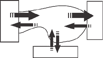
Figure 4 Diagram showing the in-scattering and out-scattering electron in and out of the
electrodes and the virtual phase-breaking contact
5. The Poisson equation
As anticipated in Section 2, the Hartree potential needed for the SCC iteration of
the Kohn–Sham equations is computed by solving the Poisson’s equation with the
appropriate boundary conditions imposed by the contacts. The Poisson’s equation for
the mean field electrostatic potential should be written as:
2
V
el
+V
ions
=−4
i
n
0
i
r +n
i
r +q
i
r −R
i
+ boundary conditions
(32)
where V
el
and V
ions
are respectively the contribution from the electrons (treated in mean
field approximation) and the ions to the total electrostatic potentials, and q
i
are the ionic
charges. The usual boundary condition used to solve the Poisson equation in DFT is that
the potential vanishes at infinity. This gives the familiar solution for the electrostatic
potential of a point charge, q,asq/r −r
, and the usual form for the Hartree energy.
In transport problem the boundary conditions are more likely imposed by the applied
potentials.
In the DFTB implementation the self-consistent potential is related to the density
fluctuations nr. The effective potential for the reference density n
0
is included in H
0
and E
rep
n
0
of Equation (1). Therefore, by linearity, we split the Poisson’s Equation (32)
into two equations, one for the ionic part plus the reference density:
2
V
0
el
+V
ions
=−4
i
n
0
i
r +q
i
r −R
i
(33)
and the other for the self-consistent correction:
2
V
2
el
=−4
i
n
i
r (34)
When solved with the usual boundary condition, Equations (33) and (34) give the
electrostatic field included in the usual DFTB calculations. However, Equation (34) is
solved using the boundary conditions imposed by the device. These conditions arise from

The gDFTB tool for molecular electronics 215
the natural requirement that deep inside the contacts the effective potential for the Kohn–
Sham equations must correspond to the bulk electrochemical potentials. Therefore, at
the boundaries between the device region and the contacts, the potential must match the
intrinsic effective bulk potential (which originates from any equilibrium charge density)
shifted by the applied bias. At the device-contacts interfaces, C
/S
, the potential must
satisfy
V
2
S
r
C
/S
=V
2
C
bulk
r
C
/S
+V
(35)
where V
is the applied external potential to the -contact. The decoupling of Equa-
tions (33) and (34), which at first may seem arbitrary, is actually a good approximation
since the reference density is taken as that of the neutral atoms and therefore can-
cels with the ionic charges. On the contrary, the excess density produces a long-range
Coulomb field that should respect the boundary conditions imposed by the device. For
example, the charge which accumulates on the contact surfaces must be consistent with
the applied bias.
Within the gDFTB approach, the Poisson equation is solved in real space using
a three-dimensional multi-grid algorithm applied to a general linear, non-separable,
elliptical PDE. The Poisson equation is just a particular case of this kind of equation,
which has the general form
i
c
ii
r
2
Vr
x
2
i
+c
i
r
Vr
x
i
+crVr = r (36)
where Vr is the unknown solution potential. The previous equation simply reduces to
the Poisson equation if the coefficients are taken such that c
i
r =cr =0 and c
ii
r =
−1/4 at all the points r of the three-dimensional box in which the equation itself
is discretized. The general equation (36) has a great flexibility. Indeed, the possibility
of setting the coefficients to different values in different regions of the solution space
is the fundamental feature which allows us to impose Dirichlet boundary conditions
on arbitrary shaped three-dimensional surfaces, such as planar or cylindrical gates, and
handles easily even four terminal geometries.
A Dirichlet boundary condition simply consists of imposing a value for the solu-
tion potential on a defined spatial region. Consequently, such a boundary condition
can be set by imposing in the spatial region occupied by the metallic gate contact,
c
ii
r = c
i
r =0 cr = 1 and Vr = r/cr. The charge density r is in turn
suitably initialized to the appropriate value, for instance, of an external gate field. The
region occupied by the gate can obviously have any arbitrary shape, since the boundary
condition is simply reduced to the initialization of a numerical function on a subset of
points on which the equation has been discretized.
In the remaining regions of the solution box, where the metallic gate is not present, the
coefficient are suitably initialized in order to obtain the effective Poisson Equation 34,
and, at the same time, the charge density is evaluated starting from the atomic charge
fluctuations projected on the real-space mesh.
Once the computation of V
2
el
r is done, it is projected back into the local orbital basis.
The mesh is usually chosen as a trade-off between accuracy and computational speed.
However, the ansatz (5) for the atomic charge density gives quite smooth functions and
usually convergent results are obtained with a mesh spacing of 0.5 atomic units.
216 A. Pecchia et al.
6. Applications to molecular conductance
In this section we show results of self-consistent computations of the I-V characteristics,
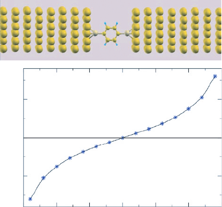
charge density and potential of molecular systems bridging metal contacts. Benzene-
dithiol, shown in Figure 5, is a simple and important test system much studied as a
test-bed reference for comparisons between theory and experiments.
For such system we find that the potential drops almost linearly across the molecular
bridge. The I-V characteristics shown in Figure 5 exhibits an ohmic behavior at small
bias which turns into a superlinear behavior beyond 2 V. The ohmic behavior owes to
a relatively high conductance also due to the position of the highest occupied level of
the molecule (HOMO), lying at 1.0 eV below E
F
.
Aviram and Ratner proposed in 1974 to realize a diode with a donor--acceptor
molecule connected at either end to metallic leads [1]. The new aspect of this idea was
that the combined system of electrons and leads could support a continuous sequence of
electron transfer processes. For the particular setup considered, the current–voltage (I-V)
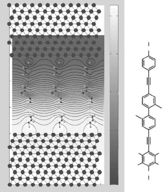
characteristic was predicted to be the one of a rectifier. More recently a small rectification
ratio was demonstrated in a break-junction experiment [27] for a single molecule. The
molecule is a variation of a Tour wire, asymmetrically doped by fluorination of a
benzene ring, as shown in Figure 6. The two rings are separated by an insulating bridge
of diphenyl, where the insulation is produced by the break of conjugation due to the
tilting angle between the two benzene rings of the bridge.
The self-consistent potential for an applied bias of 2.0 V is shown in Figure 6. From
the isolines it is possible to see that the potential drops non-linearly across the molecule,
Voltage bias (volt)
Current (amp)
5e–06
–5e–06
–3 –2 –1 0 1 2 3
0
Figure 5 Diagram showing a di-thio-phenyl molecule bridging two Au contacts and the
calculated I-V characteristics
The gDFTB tool for molecular electronics 217
30
20
10
–10
–20
–5 0 5 10 15 20
0
0.5
1
1.5
2
0
S
F
F
S
F
F
Figure 6 Self-consitent potential of a Tour wire between Au contacts
with a larger drop at the insulating bridge. The computed I-V characteristics do not
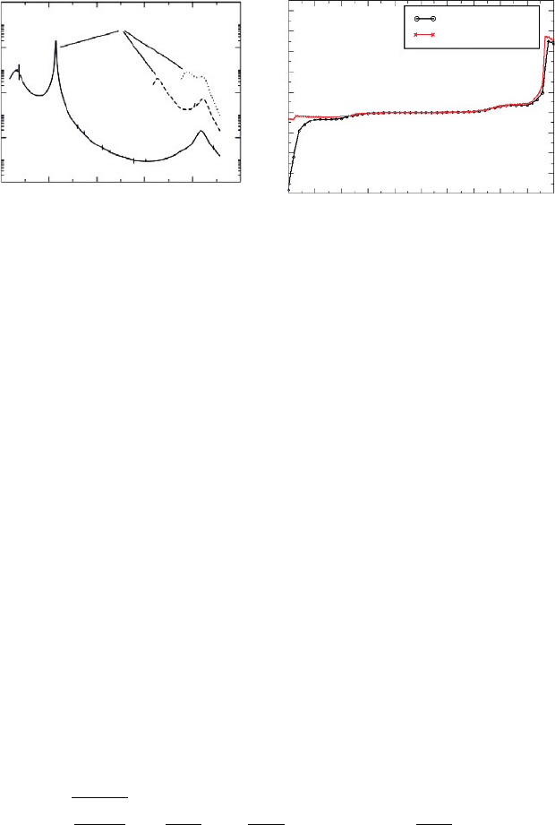
show relevant rectification within the bias range between −2 and +2 V. The computed
DFT eigenstates predict the HOMO level nearly in resonance with the Au Fermi level
at V =0 . The feature at −48 eV is instead related to the local density of states of the
contacting Au lead, as it is not affected by the applied bias. As the bias increases more
resonances enter in the injection window, as shown in the left panel of Figure 7. This
produces the staircase-like I-V characteristics shown in the right panel of Figure 7. Such
steps are also observed experimentally, although at different voltages.
The difficulty of making accurate theoretical predictions, in agreement with experi-
mental findings, is due to the high sensitivity on the precise position of the molecular
energy levels, which are very difficult to predict using just DFT calculations. As dis-
cussed in Section 9, correction for the exchange and correlation energies is necessary
for quantitative results. It is worth stressing that in transport calculations it is not just
the magnitude of the energy gap that matters, but also the absolute position of the
molecular energy levels with respect to the Fermi level of the metal, providing the
reference injection energy.
218 A. Pecchia et al.
Symmetric molecule H/H
Asymmetric molecule H/F
I (μA)
1.0
0.8
0.6
0.4
0.2
0.0
–0.2
–0.4
–0.6
–2.0
–1.0
0.0
1.0
2.0
Bias (V)
0.01
0.0001
1e–06
Transmission
1e–08
1e–10
–7 –6.5 –6 –5.5 –5 –4.5
HOMO
2.0
V
0.5
V
0.2
V
E (eV)
Figure 7 Transmission probability and computed current for the symmetric and asymmetric
Tour wire
7. Analysis of IETS spectra
An IETS spectrum is formally defined as the second derivative of I vs. V . As such
spectra are obtained at very low temperature (usually 4.2 K) only phonon emission is
possible. When the applied bias matches a phonon frequency an additional channel of
tunneling assisted by phonon emission opens up. This corresponds to a barely visible
kink in the I-V characteristics, but it can be amplified as a peak in the second derivative.
The assignment and interpretation of the spectra are not without difficulties. The spectra
are usually assigned with the help of IR, Raman and HREELS results for monolayers
of the molecule in question, or even isolated molecules. However, the interaction with
the substrate and the absence of definite selection rules means that IETS may exhibit
markedly different spectra from these other techniques and the characteristics of these
spectra are difficult to predict. Theoretical simulations are necessary in order to interpret
the measured IETS spectra [15, 28, 29].
To obtain the spectrum we calculate the coherent and incoherent current at T = 0,
using Equations (28) and (29). The calculation of the incoherent component requires
an explicit evaluation of the electron–vibration coupling matrices,
q
v
, obtained by
expanding the TB Hamiltonian to first order in the atomic displacements. The couplings
are then expressed in terms of derivatives of the Hamiltonian and the overlap matrices,
therefore without fitting parameters [30, 31], as
q
v
=
2
q
M
q
H
v
R
−
H
R
S
−1
H
v
−H
S
−1
!H
v
!R
e
q
(37)
where R
are atomic displacements, M
q
the atomic masses and e
q
the vibrational
mode eigenvectors. The relevant self-energy is evaluated within the first order Born
approximation, as
<>
el−ph
= i
q
2
d
q
G
<>
−
q
D
<>
0q
(38)
The gDFTB tool for molecular electronics 219
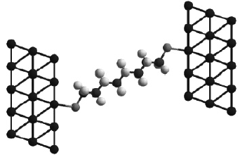
Figure 8 Relaxed Alkanethiol geometry between Au contacts
where the D
<>
0q
are the correlation functions related to the vibrational modes,
assumed Einstein oscillators in thermal equilibrium with a bath,
D
<>
0q
=−2iN
q
+1" ±
q
+N
q
∓
q
(39)
The geometry of the molecule in the junction, shown in Figure 8, is determined in
two steps. First, an optimized geometry is obtained for octanethiol chemisorbed through
the terminal sulfur to a single Au(111) surface. Periodic boundary conditions are used;
however, the chemisorbed molecules were sufficiently far apart to be considered isolated.
The geometry for the full electrode–molecule–electrode system was then generated by
symmetrizing about a point of inversion between the C4–C5 bond to give octanedithiol
bound to two co-facial Au(111).
The computed conductance of such system agrees with a model which assumes that
approximately 10,000 molecules are sampled in parallel within the nanopore device
used in the experiment [5].
The gDFTB code reproduces, to a reasonable extent, experimentally observed vibra-
tional frequencies for octanedithiol chemisorbed on Au [30]. The electrodes produce
a significant perturbation in the character of the molecule and as a consequence the
vibrational modes associated with the extremities of the molecule differ in frequency
from modes of the same character associated with the central region. For example, the
C–H symmetric stretching modes occur at different frequencies for the modes associated
with the central region (0.368 eV) and the extremities (0.348 eV).
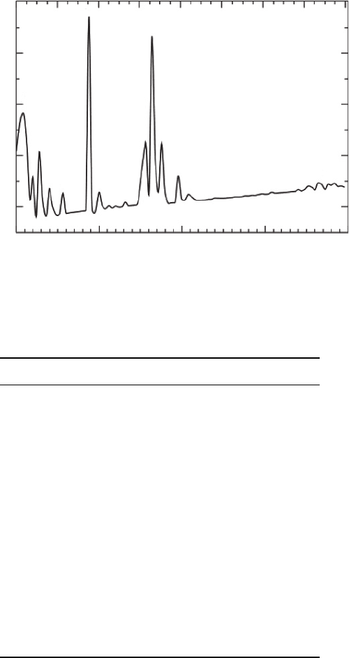
This is reflected in the calculated IETS spectra for octanedithiol, shown in Figure 9
with the peaks assigned as shown in Table 1. Unlike IETS, the spectroscopies used to
assign IETS spectra of octanedithiol (IR, Raman, HREELS) all have specific selection
rules. It has been observed previously that in IETS spectra both IR-active modes and
Raman-active modes can be seen as well as additional modes, although not all IR-active
modes and Raman-active modes may be seen. This complex relationship between what is
observed in IETS and what is observed in other spectroscopic techniques means that for
a system of the complexity of octanedithiol a complete assignment of the IETS spectra
from IR, Raman and HREELS is difficult to achieve. For instance, in the experimental
IETS spectra for octanedithiol [5] there were a number of unknown peaks attributed to
Si
3
N
4
impurities.
Indeed, according to our calculations, relevant signal from molecular modes in the
high frequency range (above 2000 cm
−1
) should not be expected. On the other hand,
220 A. Pecchia et al.
0
0
–2e–05
4e–05
2e–05
0
0.1 0.2 0.3 0.4
400 800 1200 1600 2000 2400 2800 3200
d
2
I/dv
2
(A/ V
2
)
1
2
3
4
5
7
8
9
10
11
6
12
13
14
15
Voltage (V)
Frequency (cm
–1
)
16
17
18
Figure 9 Simulation of the IETS for the octanedithiol (hcp bonding site). Numbers for peaks
are related to modes of vibration in Table 1
Table 1 Principal peaks in the calculated IETS spectrum
Peak Voltage (V) mode
10008 S–C–C out-of-plane wag
20017 S–C–C out-of-plane wag
30033 Au–S stretch
40044 S–C–C scissor
50060 C–C–C scissor
60083 C–S stretch
70111 CH
2
in-plane rock (extremities)
80121 CH
2
in-plane rock (central)
90135 CH
2
in-plane rock (central)
10 0150 CH
2
in-plane rock (all)
11 0157 C–C stretch
12 0164 C–C stretch
13 0180 CH
2
scissor (extremities)
14 0196 CH
2
scissor (central)
15 0212 CH
2
out-of-plane wag (all)
16 0217 CH
2
out-of-plane wag (all)
17 0348 C–H stretch sym (extremities)
peaks 1, 2 and 5 nicely correspond to observed, but not clearly assigned, features [5, 31].
These are low frequency modes (Table 1), the first of which can be described as a
rigid out-of-plane oscillation of the four central CH
2
-groups, the second as a rigid and
symmetric out-of-plane oscillation of the two C–C–C–S backbones. The fifth mode is

The gDFTB tool for molecular electronics 221
associated to the longitudinal oscillation of the CH
2
–CH
2
subunit pairs. Overall the
calculated spectra reflects qualitatively the experimental findings, giving the largest
signal from the backbone vibrational modes in the range 1000–1500cm
−1
.
8. Power dissipation in molecular junctions
A relevant quantity for technological applications is the amount of power dissipated in
the molecule due to inelastic phonon emission, which can be obtained by considering the
virtual contact current, as discussed, for instance, in [30]. This is an important quantity
since it is related to thermal dissipation and therefore to the stability of the molecule
under applied bias. The power dissipated is given by the net rate of energy transferred
to the molecule and can be calculated using the virtual contact current as
W =
2
h
+
−
Tr
<
ph
G
>
−
>
ph
G
<
d (40)
simply representing the average energy transfer occurring at the virtual contact.
The power dissipated can be used to compute for the rate of phonon emission. This
can be done by first observing that Equation (40) can be expressed as a sum over the
individual vibrational modes, W =
W
q
, allowing to compute the power dissipated in
each mode [30]. In order to take into account for the non-equilibrium phonon population
of the molecular modes we set up a phenomenological rate equation. The rate of phonon
emission can be defined as R
q
N
q
=W
q
/
q
(the energy emitted divided by the phonon
energy), which is a function of bias and phonon population. The rate R
q
is actually the
net rate of phonon emission, also including the absorption rate due to assisted tunneling
and electron–hole pair production, very important in metal contacts. In order to compute
the phonon population of the vibrational modes a rate equation can be written, including
the rate of emission and dissipation into the leads, as
dN
q
dt
=R
q
N
q
−J
q
N
q
−N
0
q
T =0 (41)
where J
q
is the rate of phonon dissipation and N
0
q
T is the equilibrium thermal
distribution of phonons, which is established without applied bias. Under stationary
condition, Equation (41) can be used to compute the non-equilibrium phonon population.
For the alkanethiol discussed in the previous section most of the power is emitted in the
C–C stretching modes, for which we have computed an average of 10 pW per mode. C–S
and S–Au modes adsorb approximately 8 pW. The total power emitted in the molecule
under this simple stationary model is 0.16 nW at the applied bias of 2.0 V, rising with
an approximately linear behavior. The amount of power dissipated in such molecule is
actually very small and does not affect considerably the phonon population.
To show the effect, we can consider another molecule, di-thio-phenyl, in which the
power dissipation is much larger owing to a larger incoherent current. The analysis
is restricted to those vibrational modes which give non-negligible incoherent electron–
phonon scattering [32], having frequencies of
q
= 756, 1147, 1182, and 1754 cm
−1
,
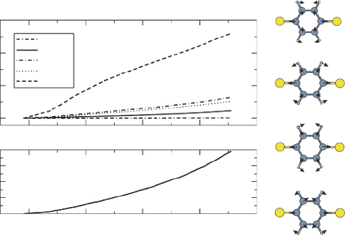
respectively. The molecule and its vibrational modes are represented in Figure 10.
The coupling of the vibrational modes with the reservoirs gives a phonon decay rate
J
q
≈10
13
Hz.
222 A. Pecchia et al.
600
500
400
300
0.8
0.6
0.4
0.2
0
0.2 0.4 0.6 0.8
0.2 0.4 0.6 0.8
Bias (V)
Power (nW) Temperature (K)
47 cm
–1
756 cm
–1
1749 cm
–1
1182 cm
–1
1147 cm
–1
756 cm
–1
1145 cm
–1
1182 cm
–1
1749 cm
–1
Figure 10 Effective mode temperature and total power dissipated into the molecule as a function
of bias for a reservoir temperature of 300 K. Vibrational mode representation of the most important
modes for incoherent electron–phonon scattering
Figure 10 shows the power dissipated and the equivalent temperature of each mode as
a function of applied bias for a contact temperature of 300 K. The equivalent temperature
is obtained from the Bose–Einstein distribution using the self-consistent solution of the
steady-state phonon population. It is possible to see that the highest energy modes heat
up considerably, reaching a temperature of almost 600 K, while low energy modes are
less sensitive. This is related to the larger power emitted in such modes and the fact
that the power emitted depends on the population itself. Since the lowest modes have
an equilibrium population, N
q
> 1, the net emission rate is small since emission and
absorption probabilities tend to cancel each other.
9. GW corrections and transport
As discussed above, the DFT approach is used to construct the one-particle system
Hamiltonian. The advantage is that DFT is a valid method to include several hun-
dreds of atoms which are frequently necessary to include an atomistic description of
the contacts. The main problem of DFT is related to the description of the unknown
exchange-correlation potential, usually approximated to be locally given by that of a
free electron gas of equal density. This tends to overestimate the metallic characteristics
of the molecular states, producing among the others, an underestimation of the HOMO–
LUMO gap, with relevant consequences to transport. Moreover, DFT is a ground-state
theory providing at most an exact electronic density, but it is not meant to compute
exact wavefunctions and single particle energy levels, both necessary ingredients for
tunneling calculations. In order to obtain quantitative prediction of tunneling currents
as well as correct quantitative trends it is necessary to go beyond DFT, even keep-
ing the simple single-particle description. Many attempts have been made to improve

The gDFTB tool for molecular electronics 223
the DFT calculations using hybrid functionals, correlated transport [33, 34] and self-
interaction corrections [35]. The alternative time-dependent current density-functional
scheme [36] could provide a consistent scheme to compute steady-state currents, auto-
matically including excited-state corrections.
Within the NEGF formalism electron–electron interactions contribute both to
<
and
to
r
. In a way similar to electron–phonon interactions, the contribution to
<
takes
into account phase-breaking scattering events, whereas
r
corrects for the single particle
propagator,
G
ra
E = ES −H−
ra
R
E −
ra
L
E −
ra
ee
E
−1
(42)
Since the Hamiltonian already contains a mean field DFT approximation for the electron–
electron interactions, it is important to note that
ee
must contain terms which subtract
such contributions. In fact the general theory for developing the electron–electron inter-
action starts usually from the free propagator.
The GW approximation is essentially a first order truncation of a general and system-
atic perturbative expansion of the electron–electron interactions in terms of a screened
Coulomb potential. The GW method takes its name from the characteristic form of the
self-energy [37],
ee
E =
GW
E =
i
2
−
dE
e
iE
0
+
G
0
E −E
WE
(43)
Where G
0
is the single particle Green’s function and WE is the screened Coulomb
potential, which can be expressed in terms of the bare Coulomb interaction, v, and the
generalized dielectric function, E,asWE =
−1
Ev, or in terms of the polarization
function W = v/1 −vPE.
GW
can be split into the sum of two terms so that
GW
= iG
0
v +iG
0
−1
−1v =
x
+
c
. The first term reduces to the known formula
for the exchange energy contribution of Hartree–Fock, whilst the second term is the
correlation part. Such an approximation has been proved to give essentially exact results
for a free electron gas [37] and provides very good corrections of bulk semiconductor
bandgaps [38, 39]. The method has been also applied with success to molecular systems
[40]. Unfortunately the full GW method is very expensive and many approximations are
necessary in order to increase the computational speed and make calculations feasible.
The GW correction has been efficiently implemented on the DFTB method [41]. The
key approximation of such implementation is to write the wavefunction products into
charge monopoles, as
r
v
r ≈
1
2
S
v
r
2
+
r
2
(44)
within the spirit of the Mulliken charge approximation used for the self-consitent charge
calculations (see Section 2). The exchange self-energy,
x
i
, can be computed using
x
i
=
occ
j
v
q
ij
v
v
q
ij
v
(45)
where the q
ij
are generalized Mulliken charges [41], and v
v
are the Coulomb integrals
between squared DFTB atomic orbitals. The correlation term is evaluated with a similar