Schlick T. Molecular Modeling and Simulation: An Interdisciplinary Guide

Подождите немного. Документ загружается.

492 14. Molecular Dynamics: Further Topics

Tensor T

Account of these modiﬁed particle interactions due to solvent structure requires

formulation of a conﬁguration and momenta-dependent hydrodynamic tensor T

to express the instantaneous effective solute force. This is because each atom’s

force changes the solvent ﬂow, and this in turn affects forces on other atoms

through the frictional forces affecting them. The tensor T is related to D by the

T factor (eq. (14.43)below).

Various expressions for hydrodynamic tensors are derived from hydrodynamic

theories (due to Kirkwood and Riseman, Oseen, Burgers, and others) so as to de-

scribe the effective velocity perturbation term, ΔV

, as the product of the tensor

and force, T(X

) F (X

). Typically, the dependence of the tensor on momenta is

ignored, and only conﬁguration-dependent effects are considered. The governing

BD equations that include hydrodynamic interactions then become:

X(t)=T(X) F (X(t)) + k

T ∇

· T(X)+R

(t) , (14.42)

where the gradient term ∇

· T(X) is the vector with components i given by



∂T

)/∂X

The Oseen and Rotne-Prager tensors expressed below have the favorable prop-

erty that the derivative of the tensor with respect to the displacement vector is

zero, a term omitted in the BD propagation scheme of eq. (14.39)[367]. These

tensors have been derived for polymer systems modeled as hydrodynamic (spher-

ical) beads of radius a immersed in a ﬂuid of viscosity η [1407]. For a polymer

system of N beads, the diffusion tensor D is then a conﬁguration-dependent,

symmetric 3N ×3N matrix in which each 3 ×3 subblock

is deﬁned as:

D =

⎛

⎜

⎝

... D

.....

... D

⎞

⎟

⎠

;

=(k

T) T

. (14.43)

Box 14.2 outlines the principles on the basis of which the tensor approxima-

tions are derived.

The frictional coefﬁcient ζ introduced in the derivation of Box 14.3 can be re-

lated to the Langevin parameter γ by: ζ = γm if all beads have the same mass

m. In fact, we can approximate roughly the reduction of the effective total fric-

tion for a polymer due to hydrodynamic effects using the Kirkwood-Riseman

(KR) approximation for bead hydrodynamics based on the Oseen tensor [966].

See Box 14.3 for this approximation.

Box 14.2: Derivation of Tensor Expressions

For macromolecules in solution, the velocity of the solvent at a polymer segment differs

from the velocity of the bulk solvent since the polymer alters the local ﬂow. The solvent

motion can thus be considered as an applied force. Let u

be the velocity of a polymer

14.5. Brownian Dynamics (BD) 493

particle (e.g., bead), v

be the velocity of the solvent at that particle, and v

be the velocity

of the bulk solvent. Then v

− u

represents the net velocity, proportional to the effective

force on the solvent at particle i:

= −ζ (v

− u

), (14.44)

where ζ is the translational friction coefﬁcient of a particle. For example, ζ =6πηa for

a bead of radius a and solvent viscosity η; assume for simplicity that ζ is the same for all

beads. The velocity at the ith bead can be written as v

plus some perturbation due to all

other segments:

= v



j=i

. (14.45)

By inserting eq. (14.45) into eq. (14.44), we have:

= −ζ

⎛

⎝



j=i

− u

⎞

⎠

= −ζ (v

− u

) − ζ



j=i

. (14.46)

It follows that

+ ζ



j=i

= −ζ (u

− v

). (14.47)

This equation is the basis for deriving the hydrodynamic tensor T, an equation that must

be solved to ﬁnd the net force for a given system.

Oseen Tensor

One of the simplest hydrodynamic tensors is the Oseen tensor, developed by Os-

een and Burgers (circa 1930) for the hydrodynamic interaction between a point of

friction and a ﬂuid, deﬁned as:

⎧

⎨

⎩

6πηa

3×3

i = j

8πηr



3×3



i = j

. (14.48)

Here r

denotes an interbead distance vector, and r

is the corresponding scalar

distance. The expression for i = j is the ﬁrst term in an expansion corresponding

to the pair diffusion for an incompressible ﬂuid in inverse powers of r

Rotne-Prager Tensor

Another term in the expansion produces the Rotne-Prager hydrodynamic tensor

. For nonoverlapping beads (r

> 2a), this matrix is deﬁned as [1071]:

⎧

⎨

⎩

6πηa

3×3

i = j

8πηr



3×3





3×3

−



i = j

(14.49)

494 14. Molecular Dynamics: Further Topics

Note that both tensors are a generalization of the scalar Langevin friction term

expressed in terms of the γ set according to Stokes’ law.

Box 14.3: Approximation of The Effective BD Friction Coefﬁcient

In the absence of hydrodynamic interactions (the “free-draining” limit), effective friction

constant f

is the sum of the friction constants of the N

individual beads, i.e., f

ζ = N

(γm). The Kirkwood-Riseman (KR) equation for f

, which approximately

incorporates hydrodynamic interactions, can be written as:

6πηN



i=j





, (14.50)

where 1/r

 is the mean inverse distance between beads i and j averaged over an en-

semble of conﬁgurations. Thus, the KR approximation is based on a preaveraged Oseen

conﬁguration tensor [966]. If we use Stokes’ law to set ζ as 6πηa, we obtain:



i=j





. (14.51)

Thus, the denominator of this expression reﬂects the reduction by hydrodynamics of the

effective friction from the reference value of N

ζ. This approximation has been used to

estimate hydrodynamic effects for long DNA [1037].

14.5.5 BD Propagation Scheme: Cholesky vs. Chebyshev

Approximation

Once the matrix D is formulated at each step n of the BD algorithm from

the hydrodynamic tensor (eq. (14.43)) the random force R must be set to sat-

isfy eq. (14.40). This is actually the computationally intensive part of the BD

propagation scheme when hydrodynamics interactions are considered.

The traditional way, based on a Cholesky decomposition of D (see [280]and

Box 14.4) increases in computational time as the cube of the system size, since

a Cholesky factorization of D is required at every step. The alternative approach

based on Chebyshev polynomials proposed by Marshall Fixman [404] only in-

creases in complexity roughly with the square of the number of variables. See

Box 14.4 for details.

Essentially, both methods for determining the random force R ﬁrst compute a

3N-vector Z from a Gaussian distribution so that

Z

 =0, Z

 =2Δtδ

;

(the indices run from 1 to 3N). The second step is different. In the Cholesky-

based approach, R is computed as R

= S

Z,whereS is the Cholesky factor of

D. In the Chebyshev procedure, we compute the random force vector instead as

14.5. Brownian Dynamics (BD) 495



Z,where



S is the square root matrix of D, and the product is computed

as a series of Chebyshev polynomials (see Box 14.4).

A recent application of the Chebyshev approach for computing the Brownian

random force in simulations of long DNA demonstrates computational savings for

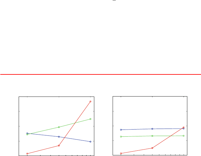
large systems [1119]. Figure 14.14 compares the percentage CPU work required

for the systematic versus hydrodynamic forces in BD simulations of DNA mod-

eled as macroscopic hydrodynamic beads using the Cholesky versus Chebyshev

approaches. The ﬁgure also shows the total CPU time required to simulate 10 ms

in both cases.

We see that for the largest, 12,000 base-pair DNA system studied, the

Chebyshev approach is twice as fast. The overall speedup is not more dramatic

since the system size (in terms of beads) is relatively small.

Perhaps more signiﬁcantly, the Chebyshev alternative to the Cholesky factor-

ization also opens the door to other BD protocols (such as the recent inertial BD

idea [106,107]) and is crucial to BD studies of ﬁner macroscopic models of DNA,

such as residue-based rather than bead-based.

Finally, note that once the BD computational bottleneck is reduced to electro-

statics and hydrodynamics (roughly O(N

) for both), fast electrostatic methods,

such as described in Chapter 10, will help accelerate such BD computations

further.

Box 14.4: BD Implementation: Cholesky vs. Chebyshev Approach

In the Cholesky approach to computing the random force to satisfy the properties of

eq. (14.40), the Cholesky decomposition of the diffusion tensor D is determined:

D = SS

where S is a lower triangular matrix. The desired vector R

is then computed from the

following matrix/vector product:

= S

Z. (14.52)

It can be easily shown that this R

satisﬁes R

)

 =2D

Δtδ

, as desired.

Note that the Cholesky decomposition of D can be written in closed form as

the following procedure for determining the elements of S, s

,rowbyrow(i.e.,

,...s

3N 3N



−



i−1

k=1



1/2



−



j−1

k=1



i>j

. (14.53)

An advantage of the Cholesky approach is that the factors can be reused. Thus, it is

possible to reduce the overall cost of the BD simulation by less-frequent updating of the

hydrodynamic tensor; parallelization of some of the numerical linear algebra tasks can

also further accelerate the total computational time [577,607].

The Chebyshev alternative was proposed over a decade ago by Marshall Fixman [404]

and recently applied [605, 681, 1119]. Instead of a Cholesky decomposition D = SS

496 14. Molecular Dynamics: Further Topics

Fixman suggests to calculate R from the relation



Z, (14.54)

rather than eq. (14.52)where



S is the square root matrix of D:

D =



This idea is based on expanding the matrix/vector product



SZ as a series of Chebyshev

polynomials which approximate the function

√

x on some given interval believed to

contain eigenvalues. This calculation requires about O(N

) operations, thus reﬂecting

substantial savings with respect to the Cholesky approach.

The details of computing the expansion of R in this Chebyshev approximation were

recently given in the appendix of [1119] in an application of BD to supercoiled DNA. See

also [605,681] for other applications. The Chebyshev implementation requires determining

bounds on the maximum and minimum eigenvalues of D

and then computing an expan-

sion of desired order (according to some error criterion) of R in terms of polynomials, with

coefﬁcients determined for the square-root function.

100 200 400

days

120

CPU/10ms

Force

Hydro.

3 kbp 6 kbp 12 kbp

100 200 400

100

CPU

Work

120

CPU/10ms

Hydro.

Force

3 kbp 6 kbp 12 kbp

BD with Cholesky factorization BD with polynomial expansion

Figure 14.14. Computational complexity for BD schemes with hydrodynamics as obtained

for a bead model of DNA using Cholesky and Chebyshev approaches for computing the

Brownian random force. The fraction of CPU associated with the hydrodynamics and sys-

tematic force calculations is shown in each case (% scales at left) as a function of system

size, with corresponding total number of days required to compute a 10 ms trajectory

(shown with the scale at right). Computations are reported on an SGI Origin 2000 machine

with 300 MHz R12000 processor [1119].

14.6 Implicit Integration

A reasonable approach for allowing long timesteps is the use of implicit integra-

tion schemes [447]. These methods are designed speciﬁcally for problems with

disparate timescales where explicit methods do not usually perform well, such

14.6. Implicit Integration 497

as chemical reactions [495]. The integration formulas of implicit methods are

designed to increase the range of stability for the difference equation.

Typically, implicit methods work well when the fast components are rapidly

decaying and largely decoupled from the slower components. This is not the case

for biomolecules, where vibrational modes are intricately coupled and the fast

motions are oscillatory.

14.6.1 Implicit vs. Explicit Euler

To illustrate the use of implicit methods, we consider a simple example for the

solution of the general differential equation

Y (t)=F[Y (t)] , (14.55)

where Y =(X, V ) is a vector and F is a vector function. The Newtonian system

of equations (13.7, 13.8) can be written in this form with the composite vector

Y =(X,

X) and the function

F[Y (t)] = [V (t), −M

−1

∇E (X(t))] .

The implicit-Euler (IE) scheme discretizes eq. (14.55)as

n+1

− Y

)/Δt = F(Y

n+1

) , (14.56)

while the explicit Euler (EE) analog has the different right-hand-side:

n+1

− Y

)/Δt = F(Y

) . (14.57)

In the former case, the solution Y

n+1

is derived implicitly, since F(Y

n+1

) is not

known and must be solved by some procedure. In the latter, the solution can be

explicitly formulated in terms of quantities known from previous steps.

Though the explicit approach is simpler to solve, it imposes a severe restriction

on the timestep. Implicit schemes can yield much better stability behavior for

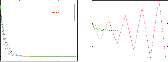
‘stiff’ problems [495]. This can be seen in Figure 14.15, where we solve the one-

dimensional problem y



= −ay, a > 0, whose exact solution is y =exp(−at)

by the implicit and explicit Euler methods.

It can be shown that the former gives the recursion relation

= y

/(1 + aΔt)

while the latter gives

= y

(1 −aΔt)

The IE scheme is always stable since aΔt>0, but EE requires that aΔt<2.

The experience with implicit methods in the context of biomolecular dynamics

has been limited and rather disappointing (e.g., [604,1437]). The disappointment

stems from three basic reasons: intrinsic damping, large computational demands,

and resonance artifacts.

498 14. Molecular Dynamics: Further Topics

0 5 10 15 20

0.2

0.4

0.6

0.8

a Δt = 0.5 a Δt = 2.2

Exact

0 5 10 15 20

−4

−3

−2

−1

Solution y(t )

Figure 14.15. Implicit (IE) and explicit (EE) Euler solutions to the one-dimensional dif-

ferential equation y



= −ay with a>0 are shown. They indicate stability of IE at

small and large timesteps but growing instability of EE with time if the timestep is not

sufﬁciently small. Here we use y

=1and two ratios for aΔt (0.5, left, and 2.2, right).

The corresponding IE and EE solutions (see text) yield, respectively, y

=1/(1.5)

and

=(0.5)

for the smaller timestep, and y

=1/(3.2)

and y

=(−1.2)

for the

larger timestep.

14.6.2 Intrinsic Damping

Despite the high stability of the IE discretization, the IE scheme is nonconserva-

tive and exhibits intrinsic damping. For system (14.27), the IE discretization is:

M(V

n+1

− V

)/Δt = F (X

n+1

) − γMV

n+1

+ R

n+1

− X

)/Δt = V

n+1

. (14.58)

This scheme was introduced to molecular dynamics with the Langevin restoring

force over a decade ago [992, 1132], but its γ and timestep-dependent damping

[992, 1107] ruled out general applications to biomolecules. This was concluded

from the tendency of the scheme to preserve ‘local’ structure (as measured by

ice-like features of liquid water [1120], the much slower decay of autocorrelation

functions [298, 927], or lower effective temperature [298]).

Thus, at large timesteps, the IE method was numerically stable but behaved

like an energy minimizer. Still, the IE scheme was incorporated as an in-

gredient in dynamic simulations of macroscopic separable models in which

high-frequency modes are not relevant [1105, 1125, 1127, 1128], and in en-

hanced sampling schemes with additional mechanisms that counteract numerical

damping [298,299,513].

14.6.3 Computational Time

In addition to the general damping problem, there is often no net computational

advantage in implicit schemes. Each timestep, albeit longer, is much more expen-

sive than an explicit timestep because a subproblem must be solved at each step.

14.6. Implicit Integration 499

This subproblem arises because the solution for X

n+1

and V

n+1

cannot be solved

in closed form (i.e., in terms of previous iterates) as in explicit schemes. Note that

the (n +1)iterates of V or X appear on both the right and left-hand sides of

eq. (14.58). Solving for X

n+1

requires solution of a nonlinear system.

It has been shown that this solution can be formulated as a nonlinear optimiza-

tion problem and solved using efﬁcient Newton schemes [992,1437], such as the

truncated-Newton method introduced in Chapter 11.Asfastastheminimization

algorithm might be, the added cost of the minimization makes implicit schemes

competitive with explicit, small-timestep integrators only at very large time-

steps, a regime where reliability is questionable given the damping and resonance

effects.

14.6.4 Resonance Artifacts

Resonance, the third problem associated with implicit methods, is relevant to

implicit schemes since large timesteps may yield stable methods [821].

A detailed examination of resonance artifacts with the implicit midpoint (IM)

was described in [821]. IM differs from IE in that it is symmetric and symplectic.

It is also special in the sense that the transformation matrix for the model linear

problem is unitary, partitioning kinetic and potential-energy components identi-

cally. For these reasons, several researchers have explored the application of IM

to long-timestep dynamics [468,632,1186, 1187].

IM Analysis

The IM discretization applied to system (14.27)is:

M (V

n+1

− V

)/Δt =

−∇E

+ X

n+1

) −

γM

+ V

n+1

)+R

n+1

− X

)/Δt =(V

+ V

n+1

)/2 . (14.59)

This nonlinear system can be solved, following [992], by obtaining X

n+1

as a

minimum of the “dynamics function” Φ(X):

Φ(X)=

γ

(X − X

)

M (X − X

)+(Δt)



X + X



, (14.60)

where

= X

+(ΔtV

)/γ + M

−1

(Δt)

/(2γ),

and

γ =1+(γΔt)/2 .

Hence, for IM applied to Newtonian dynamics γ =1,andtheR

term in X

absent. Following minimization of the IM dynamics function to obtain X

n+1

,the

new velocity, V

n+1

, is obtained from the second equation of system (14.59).

An examination of the application of IM to MD showed good numerical prop-

erties (e.g., energy conservation and stability) for moderate timesteps, larger than

500 14. Molecular Dynamics: Further Topics

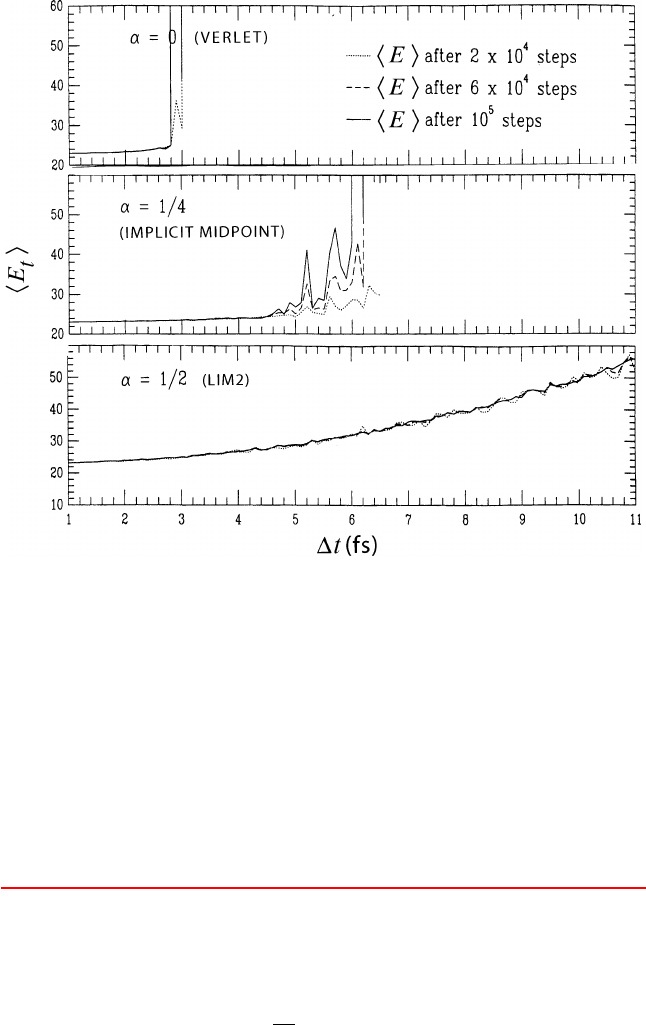
Figure 14.16. Mean total energy for a blocked alanine model as a function of the timestep,

as obtained by Verlet, implicit-midpoint, and the symplectic implicit scheme LIM2 [1437];

see [1126].

Ver let [ 821, 1437]. However integrator-induced resonance artifacts were found

to be severe as the timestep approaches half the characteristic period [821](see

Box 14.5).

Figure 14.16 shows the mean total energy for Verlet and IM for a blocked

alanine model [1126] (misnamed ‘dipeptide’ in some works). Note that Verlet

becomes unstable around 2.8 fs (recall Table 14.2 for reference linear-analysis

values), and IM exhibits resonance peaks around 5.2 and 5.7 fs and instability

around 6 fs, all near half the period of the fast motion.

Box 14.5: Analysis of Implicit-Midpoint (IM) Resonance

The linear analysis of [821] has shown that the effective angular rotation θ

eﬀ

of IM is:

eﬀ

Δt

tan

−1

(ωΔt/2) . (14.61)

14.6. Implicit Integration 501

Recall that the corresponding value for the Verlet scheme (eq. (14.19)) is:

verlet

eﬀ

=2sin

−1

(ωΔt/2) .

As derived above, the resonant timestep of order n:m can be obtained for the model

linear problem by using the function for ω

eﬀ

in the expression

nΔtω

eﬀ

=2πm ,

since those timesteps correspond to a sampling of n phase-space points in m revolutions.

This substitution yields for the IM scheme

Δt

n:m

tan



πm



tan



πm



. (14.62)

For n =3, 4 and m =1,wehave,forexample:Δt

3:1

√

3/ω and Δt

4:1

=2/ω

for IM. These resonance times are larger than corresponding values for Verlet:

√

3/ω and

√

2/ω, respectively. Hence IM confers better stability than Verlet.

If we consider a fast period of 10 fs (see Table 14.2), the IM resonant timesteps for

orders n =3, 4, 5, 6 are 5.5, 3.2, 2.3, and 1.8 fs, respectively, compared to 2.8, 2.3, 1.9,

and 1.6 fs for Verlet. This analysis explains the results shown in Figure 14.16.

A Family of Symplectic Implicit Schemes

The IE and IM methods described above turn out to be quite special in that IE’s

damping is extreme and IM’s resonance patterns are quite severe relative to related

symplectic methods. However, success was not much greater with a symplectic

implicit Runge-Kutta integrator examined by Janeˇziˇc and coworkers [604].

A family of implicit symplectic methods including IM and Verlet (as a special

case) was also explored in subsequent works by Skeel, Schlick, and coworkers

[446, 1126]. The family of methods can be parameterized via α (see Box 14.6).

The values α =0, α =1/2,and1/4 correspond to the Verlet, ‘LIM2’, and IM

methods, respectively. The LIM2 method appeared attractive based on the effec-

tive rotation analysis (see Box 14.6), since it should exhibit no erratic resonance

patterns; this was indeed observed in practice (Figure 14.16.) Unfortunately,

this resonance removal comes at the price of large increases in energy with the

timestep, as also seen in Figure 14.16.

These scheme-dependent resonances were concluded by the analysis in [1126]

on the basis of the effect of the parameter α on the numerical frequency of the

integrator for the system simulated. Speciﬁcally, the maximum possible phase an-

gle change per timestep decreases as the parameter α increases. Hence, the

angle change can be limited by selecting a suitable α.

The choice α ≥

, as in the LIM2 method, restricts the phase angle change

to less than one quarter of a period and thus is expected to eliminate notable

disturbances due to fourth-order resonance.

The requirement that α ≥

guarantees that the phase angle change per time-

step is less than one third of a period and therefore should also avoid third-order

resonance for the model problem.