Schlick T. Molecular Modeling and Simulation: An Interdisciplinary Guide

Подождите немного. Документ загружается.

482 14. Molecular Dynamics: Further Topics

14.4.4 Generalized Verlet for Langevin Dynamics

The Verlet algorithm can easily be generalized to include the friction and stochas-

tic terms above. A common discretization is that described by Brooks, Br¨unger

and Karplus, known as BBK [180, 967]:

Generalized Verlet Algorithm for Langevin Dynamics

n+1/2

= V

+ M

−1

Δt

[−∇E(X

) − γMV

+ R

]

n+1

= X

+ΔtV

n+1/2

(14.30)

n+1

= V

n+1/2

+ M

−1

Δt



−∇E(X

n+1

) − γMV

n+1

+ R

n+1



This Langevin scheme reduces to velocity Verlet (triplet eq. (13.14)) when γ

and hence R

are zero.

Note that the third equation above deﬁnes V

n+1

implicitly; the linear depen-

dency, however, allows solution for V

n+1

in closed form (i.e., explicitly). The

superscript used for R has little signiﬁcance, as the random force is chosen

independent at each step.

When the Dirac delta function of eq. (14.28) is discretized, δ(t −t



) is replaced

by δ

/Δt.

The BBK method is only appropriate for the small-γ regime. A more ver-

satile algorithm was derived in [1293]. See also [1200] for a related Langevin

discretization.

14.4.5 The LN Method

The idea of combining force splitting via extrapolation with Langevin dynamics

can alleviate severe resonance effects — as discussed in the MTS section (and

shown in Figure 14.5 for a simple harmonic model) — and allow larger outer

timesteps to be used than impulse-based MTS schemes [93–95].

The LN algorithm based on this combination (see background in Box 14.1)

is sketched in Figure 14.8 in the same notation used for the MTS schemes. The

direct-force algorithms on the left forms the basis for the algorithms implemented

in the CHARMM [95]andAMBER[89,97,1025] programs.

Note that LN is based on position Verlet rather than velocity Verlet. If a

constrained dynamics formulation is used (e.g., SHAKE), this splitting version

requires on average two SHAKE iterations per inner loop rather than the one

required by velocity Verlet. However, we have found stability advantageous in

practice for the position Verlet scheme over velocity Verlet in the unusual limit of

moderate to large timesteps and large timescale separations [99].

14.4. Langevin Dynamics 483

0 20 40

−4

−2

Outer Timestep [fs]

Energy [Kcal/mol]

Langevin Impulse

0 5 10

−5

x 10

Outer Timestep [fs]

Energy [Kcal/mol]

Newtonian Extrapolation

Newtonian Impulse

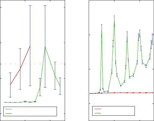
Figure 14.7. Energy means and deviations as computed over 5-ps Newtonian and Langevin

impulse and extrapolative force splitting schemes for the protein BPTI with the damping

constant γ =20ps

−1

, as functions of the outer timestep for a ﬁxed inner timestep of 0.5 fs

and medium timestep of 1 fs [1089].

Resonance Alleviation

Applications to the solvated model of the protein BPTI in Figure 14.7 show

how the Langevin extrapolative treatment alleviates severe resonances present

in impulse treatments for both Newtonian and Langevin dynamics. Newto-

nian extrapolation yields large energy increases as the timestep increases. Both

Newtonian and Langevin impulse splitting exhibit resonant spikes: beyond half

the fastest period for Newtonian impulse, and beyond the fastest period for

Langevin impulse splitting. Unfortunately, once such resonance is encountered,

good behavior cannot be restored after the ﬁrst resonant timestep. The LN com-

bination, in contrast, does not exhibit resonant spikes for this value of damping

constant, 20 ps

−1

. It stabilizes the energy growth seen for Newtonian extrapola-

tion. See also [1134] for detailed performance evaluations for a large protein/DNA

complex.

The exchange of Hamiltonian dynamics for stochastic dynamics can guarantee

better numerical behavior, but the resulting dynamics are altered. Stochastic dy-

namics are, however, suitable for many thermodynamic and sampling questions.

Small-timestep dynamics simulations can always be performed in tandem once

an interesting region of conformation space is identiﬁed.

484 14. Molecular Dynamics: Further Topics

LN Algorithm

(Direct Force Version) (Linearization Variant changes)

≡ X X

≡ X +

Δt

slow

≡−∇E

slow

)

For j =1 to k

≡ X

← X +

Δt

V X

← X +

Δt

V ;



≡



H(X

)

med

≡−∇E

med

) F

med

≡−∇E

med

) −∇E

fast

)

F ← F

med

+ F

slow

For i =1 to k

Evaluate Gaussian force R

X ← X +

Δτ

tot

← F + F

fast

(X)+R F

tot

← F −



· (X −X

)+R

V ←



V + M

−1

ΔτF

tot



/γ

X ← X +

Δτ

End

End [γ =1+γΔτ] [



= local Hessian approx.]

Figure 14.8. Algorithmic sketch of the LN scheme [95] for Langevin dynamics by extrap-

olative force-splitting based on position Verlet. The version on the left uses direct fast-force

evaluations, while the reference version on the right (only alternative statements shown)

uses linearization to approximate the fast forces over a Δt

interval. The latter requires a

local Hessian formulation,



H(X

), at point X

every time the medium forces are

evaluated. See Box 14.1 for background details.

Skeel, Izaguirre, and coworkers have also adopted the stochastic coupling [594,

595] in the context of the molliﬁed impulse method [1133] to extend the timestep

beyond half the fast period. Because their γ is yet smaller, the agreement with

Hamiltonian dynamics is better, but the largest possible outer timesteps and hence

speedup factors are reduced.

An interesting recent variation called “NML” [1242] is an extension of a LIN

[1435,1436] developed as a way to increase the timestep in standard MD integra-

tion. The idea in LIN was to use implicit integration for the low-frequency modes

and normal-mode analysis (NMA) for the high-frequency modes; Langevin rather

than Newtonian dynamics was also used to dampen resonance effects, which

limit the timestep to around 3.3 fs when all light-atom motions are consid-

ered. In NML, the costly NMA of LIN is replaced by Brownian dynamics

for the high-frequency modes to keep the fast oscillations around their equilib-

rium values; the low-frequency modes are propagated by Langevin dynamics as

in LIN.

14.4. Langevin Dynamics 485

Box 14.1: LN Background and Assessment

Background. LN arose fortuitously [93] upon analysis of the range of harmonic validity

of the Langevin/Normal-mode method LIN [1435,1436]. Essentially, in LIN the equations

of motion are linearized using an approximate Hessian and solved for the harmonic com-

ponent of the motion; an implicit integration step with a large timestep then resolves the

residual motion (see subsection on implicit methods). Approaches based on linearization

of the equations of motion have been attempted for MD [67, 603, 1209, 1280], but compu-

tational issues ruled out general macromolecular applications. Indeed, the LIN method is

stable over large timesteps such as 15 fs but the speedup is modest due to the cost of the

minimization subproblem involved in the implicit discretization. The discarding of LIN’s

implicit-discretization phase — while reducing the frequency of the linearization — in

combination with a force splitting strategy forms the basis of the LN approach [95].

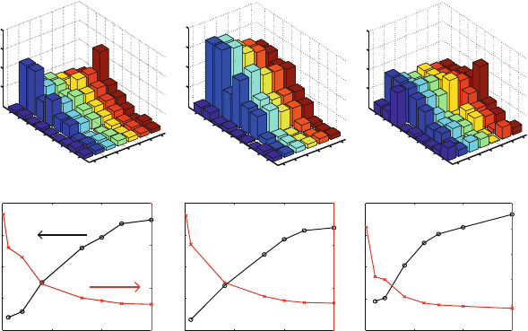
Performance: Energetics and Speedup. Performance of MTS schemes can be analyzed

by ‘Manhattan plots’, as shown in Figure 14.9 for a large polymerase/DNA system of

41,973 atoms (illustrated in Figure 14.10)[1408]; that is, differences of mean energy

components are reported as a function of the outer timestep Δt relative to STS Langevin

simulations. For three LN protocols — using different combinations of Δτ , Δt

, γ,and

bond constraints (SHAKE on or off) — these plots, along with corresponding CPU times

and speedup, show that the ﬁrst protocol has the optimal combination of low relative

error in all energy components (below 3%) and low CPU time per physical time unit. The

computational speedup factor is 4 or more in all cases.

Performance: Dynamics. The assignment of the Langevin parameter γ in the LN scheme

ensures numerical stability on one hand and minimizes the perturbations to Hamiltonian

dynamics on the other; we have used γ =10ps

−1

or smaller in biomolecular simulations.

To assess the effect of γ of dynamic properties, the protocol-sensitive spectral density

functions computed from various trajectories can be analyzed (see Figure 14.11 caption).

The densities for solvated BPTI in Figure 14.11 show how the characteristic frequencies

can be more closely approximated as γ is decreased; the densities for the large polymerase

system in Figure 14.12 show, in addition, the good agreement between the STS Langevin

and LN-computed frequencies for the same γ. This emphasizes the success of MTS in-

tegrators as long as the inner timestep is small. (Recall another illustration of this point

for butane in Figure 13.5, where the average butane end-to-end distance is shown for STS

versus MTS protocols).

Detailed comparisons of the evolution of various geometric variables (Figure 14.13)re-

ﬂect the agreement between LN and the reference Langevin simulation as well [1408]. As

expected, individual trajectories diverge, but the angular ﬂuctuations are all in reasonable

ranges. The ﬂexibility of the DNA backbone angles is expected at the base pair near the

kink induced by the polymerase [1408].

486 14. Molecular Dynamics: Further Topics

100

120

150

Temp

Evdw

Etot

Eelec

Etors

Eangle

Ebond

100

120

150

Temp

Evdw

Etot

Eelec

Etors

Eangle

Ebond

0 50 100 150

100

150

100

120

150

Temp

Ebond

Etot

Evdw

Eelec

Etors

Eangle

abc{Δτ, Δt

} = {1, 2} fs

No SHAKE

SHAKE

LN speedup factor

CPU time (days/ns)

Relative error [%]

Energy [kcal/mol] Outer timestep [fs]

{Δτ, Δt

} = {1, 2} fs {Δτ, Δt

} = {0.5, 1} fs

γ = 10 ps

−1

γ = 5 ps

−1

γ = 10 ps

−1

Outer timestep [fs]

0 50 100 150

100

150

0 50 100 150

100

150

200

250

CPU time

Speedup

Figure 14.9. ‘Manhattan plots’ for a solvated polymerase/DNA system showing the LN

relative errors in different energy components (bond, bond angle, torsion, electrostatic, po-

tential, total, van der Waals) and the kinetic temperature as a function of the outer timestep

Δt compared to single-timestep Langevin trajectories at the same Δτ,aswellascorre-

sponding speedups (scale at left) and CPU times per nanosecond (scale at right). ‘SHAKE’

refers to constraining all bonds involving hydrogen. The data for three parameter com-

bination in (a–c) are based on simulations of length 12 ps started from the intermediate

polymerase/DNA complex [1408], pictured in Figure 14.10. See also Box 14.1.

Testing and Application

Results have shown that good parameter choices for a 3-class LN scheme are

Δτ =0.5 fs, Δt

=1fs, and Δt up to 150 fs. If constrained dynamics

for the light atom bonds are used, the inner timestep can be increased to 1 fs

and the medium timestep to around 2 fs. Various biomolecular applications have

shown good agreement of LN trajectories to small-timestep Langevin simulations

and signiﬁcant speedup factors [95, 1230, 1408]. See Box 14.1 for performance

assessment of energetics, dynamics, and speedup on a biomolecule.

Recent work has tailored elements of the LN integrator to particle-mesh Ewald

protocols [97, 99, 1024, 1025]. Challenges remain regarding the most effective

MTS splitting procedures for Ewald formulations, given the fast terms present

in the Ewald reciprocal component [89, 97, 98, 1025, 1110, 1236, 1449]and

the numerical artifact stemming from subtraction of the term accounting for

excluded-nonbonded atoms pairs [89,1019,1025].

14.5. Brownian Dynamics (BD) 487

Figure 14.10. Solvated polymerase/DNA system used for evaluating LN [1408].

0 1000 2000 3000 4000

Protein

Velocity Verlet

= 5 ps

-1

=20 ps

−1

0 1000 2000 3000 4000

Water

Wave number [cm

−1

] Wave number [cm

−1

]

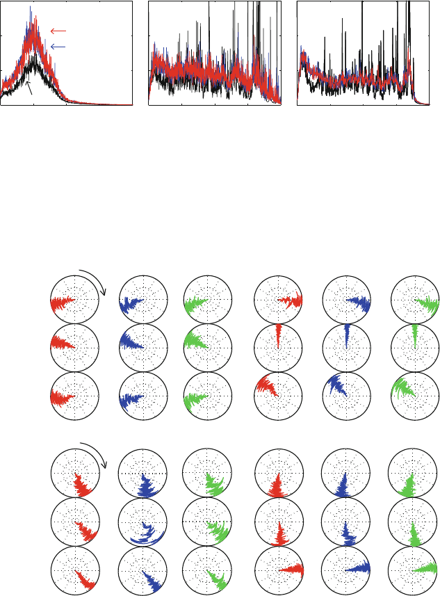
Figure 14.11. Spectral density functions calculated by Verlet and LN over 5 ps runs for a

solvated system of the protein BPTI (protein and water frequencies shown separately) at

three γ values: 0 (by the velocity Verlet scheme), 5 and 20 ps

−1

by the LN scheme [1089].

The functions are computed by Fourier transforming the velocity autocorrelation time se-

ries for each atom in the system to obtain a power spectrum for each atom. These spectra

are averaged over the water and biomolecule atoms separately for global characterization

of the motion. See [1089] for the detailed protocol. Note that the characteristic frequencies

obtained by this procedure reﬂect the force ﬁeld constants rather than physical frequencies

per se.

14.5 Brownian Dynamics (BD)

14.5.1 Brownian Motion

The mathematical theory of Brownian motion is rich and subtle, involving high-

level physics and mathematics. Important contributors to the theory include

Einstein (who explained Brownian motion in 1905) and Planck. Here we present

488 14. Molecular Dynamics: Further Topics

0 500 1000 1500 2000 0 500 1000 1500 20000 500 1000 1500 2000

Wave number [cm

−1

]

Water

DNA

Protein

LN 1/2/150 fs

BBK 1 fs

γ = 10 ps

−1

VV 1 fs

Figure 14.12. Spectral density functions calculated by the STS Newtonian (velocity Verlet)

and STS Langevin (BBK, γ =10ps

−1

) schemes versus the MTS LN scheme at

γ =10ps

−1

(triple timestep protocol 1/2/150 fs) for a solvated polymerase/DNA sys-

tem simulated over 12 ps and sampled every 2 fs. Spectral densities for the protein, DNA,

and water atoms are shown separately. See also caption to Figure 14.11.

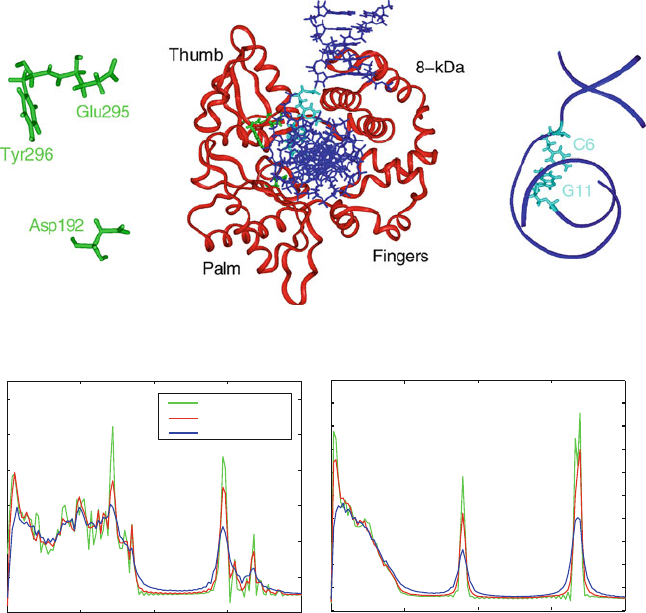
Asp192

Glu295

Tyr296

Protein φ

Protein ϕ

LN BBK VV LN BBK VV

DNA C6 DNA G11

270

Figure 14.13. Comparisons of the evolution of representative dihedral angles (from protein

φ and ψ and DNA sugar and backbone near one CG base pair) over 12 ps for the STS veloc-

ity Verlet, STS Langevin (BBK), and the MTS LN scheme for a solvated polymerase/DNA

system. The LN protocol used is Δτ =1fs, Δt

=2fs, and Δt = 150 fs, with SHAKE.

The polar vector coordinates correspond to time and angle. See Figure 14.10 for location

of residues.

14.5. Brownian Dynamics (BD) 489

the BD framework as an extension to the Langevin model presented above and

focus on numerical algorithms for Brownian dynamics. See statistical mechanics

texts, such as [853], for more comprehensive presentations.

The term Brownian is credited to the botanist Robert Brown, who in 1827 ob-

served that ﬁne particles — like pollen grains, dust, and soot — immersed in a

ﬂuid undergo a continuous irregular motion due to collisions of the particles with

the solvent molecules. Dutch physician Jan Ingenhausz was actually the ﬁrst, in

1785, to report this motion for powdered charcoal on an alcohol surface. The ef-

fective force on such particles originates from friction, as governed by Stokes’

law, and a ﬂuctuating random force.

14.5.2 Brownian Framework

Generalized Friction

Generalized frictional interactions among the particles can be incorporated into

the Langevin equation introduced in Section 14.4 using a friction tensor Z.

This matrix replaces the single parameter γ, so as to describe the action of the

solvent by:

X(t)=−∇E(X(t)) − Z

X(t)+R(t), (14.31)

where the mean and covariance of the random force R are given by:

R(t) =0, R(t)R(t



)

 =2k

TZ δ(t − t



) . (14.32)

The above relation is based on the ﬂuctuation/dissipation theorem, a fundamental

result showing how friction is related to ﬂuctuations of the random force, as-

suming the Brownian particle is randomly moving about thermal equilibrium.

This description ensures that the ensembles of the trajectories generated from

eq. (14.31) are governed by the Fokker-Planck equation, a partial-differential

equation describing the density function in phase space of a particle undergoing

diffusive motion.

The random force R is white noise and has no natural timescale. Thus, the

inertial relaxation times given by the inverses of the eigenvalues of the matrix

−1

Z deﬁne the characteristic timescale of the thermal motion in eq. (14.31).

Neglect of Inertia

When the inertial relaxation times are short compared to the timescale of interest,

it is often possible to ignore inertia in the governing equation, that is, discard the

momentum variables, assuming M

X(t)=0.Fromeq.(14.31), we have:

X(t)=− Z

−1

∇E(X(t)) + Z

−1

R(t), (14.33)

and this can be written in the Brownian dynamics form:

X(t)=−

∇E(X(t)) + R

(t); (14.34)

490 14. Molecular Dynamics: Further Topics

here D is the diffusion tensor

D = k

−1

, (14.35)

and the mean and covariance of the random force R

depend on D as:

R

(t) =0, R

(t)R



)

 =2D δ(t − t



) . (14.36)

Thus, solvent effects are sufﬁciently large to make inertial forces negligible,

and the motion is overall Brownian and random in character. This description

is effective for very large, dense systems whose conformations in solution are

continuously and signiﬁcantly altered by the ﬂuid ﬂow in their environment.

Transport Properties

Brownian theory allows us to determine average behavior, such as transport prop-

erties, for systems governed by such diffusional motion. For example, a molecule

modeled as a free Brownian particle that moves a net distance x over a time in-

terval Δt has an expected mean square distance x

 (analogous to the mean

square end-to-end distance in a polymer chain) proportional to Δt: x

∝Δt.

Einstein showed that the proportionality constant is 2D,whereD is the diffusion

coefﬁcient:

x

 =2D Δt.

Algorithms

An appropriate simulation algorithm for following Brownian motion can be

deﬁned by assuming that the timescales for momentum and position relaxation

are well separated, with the former occurring much faster. BD algorithms then

prescribe recursion recipes that displace each current position by a random force

— similar in ﬂavor to the Langevin random force — and additional terms that

depend on the diffusion tensor.

It is not always possible to neglect inertial contributions. For example, it was

shown that inertial contributions can affect long-time processes in long DNA due

to mode coupling [107]. An “inertial BD” algorithm termed IBD has been devel-

oped, tested on simple systems [106], and applied to bead models of long DNA

[107]. IBD more accurately approximates long-time kinetic processes that occur

within equilibrium ensembles, as long as the timestep is not too small.

In practice, the IBD scheme adds a mass-dependent correction term to the usual

BD propagation scheme (see below). Though IBD has an additional computa-

tional cost of a factor of two over BD, the computational complexity is the same

as for the usual BD scheme based on the Cholesky factorization (consult a numer-

ical methods textbook like [280] for the Cholesky factorization, and see Box 14.4

and below for IBD details).

14.5. Brownian Dynamics (BD) 491

14.5.3 General Propagation Framework

In general, larger timesteps are used for Brownian dynamics simulations than for

molecular and Langevin dynamics simulations. As a ﬁrst example, consider a free

particle in one dimension whose diffusion constant D is (by deﬁnition) the mean

square displacement divided by 2t:

2tD ≈|x(t) −x(0)|



over sufﬁciently long times. This diffusional motion can be simulated by the

simple scheme:

n+1

= x

+ R

, (14.37)

where the random force R is related to D by:

R

 =0, (R

)

 =2DΔt. (14.38)

This propagation scheme reproduces D over long times t; see homework

assignment 12.

Ermak/McCammon

Ermak and McCammon [367] derived a basic BD propagation scheme from the

generalized Langevin equation in the high-friction limit, where it is assumed

that momentum relaxation occurs much faster than position relaxation. For a

three-dimensional particle diffusing relative to other particles and subject to a

force F (X), the derived BD scheme becomes:

n+1

= X

Δt

F (X

)+R

, (14.39)

R

 =0, R

)

 =2D

Δtδ

. (14.40)

For reference, the IBD algorithm developed in [106] has the following mass-

dependent correction term:

n+1

= X

Δt

F (X

[F (X

n−1

)−F (X

)]+R

(14.41)

with the same random-force properties for R as above (eq. (14.40)).

14.5.4 Hydrodynamic Interactions

Various approaches have been developed to deﬁne the diffusion tensor D in these

equations. Recall from Subsection 14.2.5 that the simple Langevin formulation

offers only a simple isotropic description of viscous effects: frictional effects

are taken to be isotropic, so γ is a scalar. Furthermore, the random force R

acts independently on each particle, thereby ignoring changes in force due to the

solvent-mediated dynamic interparticle interactions.