Sandau R. Digital Airborne Camera: Introduction and Technology
Подождите немного. Документ загружается.

2.7 Colour 91
transition from the colour space of the primary colours R, G, B to the space of the
so-called standard colours X, Y, Z must be performed.
The vectors X, Y, Z are connected with the vectors R, G, B via the linear
transform
⎛
⎝
X
Y
Z
⎞
⎠
= A ·
⎛
⎝
R
G
B
⎞
⎠
(2.7-5)
with
A =
⎛
⎝
2.36460 −0.51515 0.00520
−0.89653 1.42640 −0.01441
−0.46807 0.08875 1.00921
⎞
⎠
(2.7-6)
If, analogously to (2.7-1), one writes
F = X · X + Y ·Y + Z · Z, (2.7-7)
then one obtains the following connection between the primary colour values R, G,
B and the normalized colour values X, Y, Z:
⎛
⎝
R
G
B
⎞
⎠
= A
T
·
⎛
⎝
X
Y
Z
⎞
⎠
and
⎛
⎝
r
λ
g
λ
b
λ
⎞
⎠
= A
T
·
⎛
⎝
x
λ
y
λ
z
λ
⎞
⎠
(2.7-8)
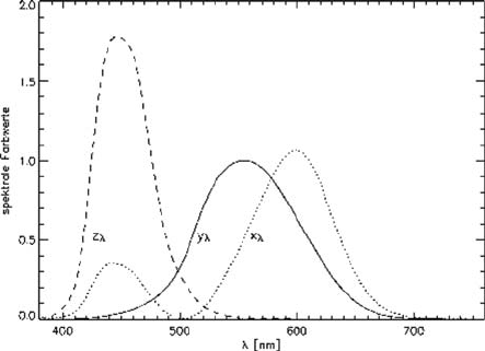
Here A
T
is the transpose of matrix A and x
λ
, y
λ
, z
λ
are the standard spectral value
functions (see Fig. 2.7-2), respectively. The normalized spectral value functions
have non-negative values and may be implemented with suitable filters.
Fig. 2.7-2 Standard spectral value functions

92 2 Foundations and Definitions
Analogously to (2.7-4), the standard colour values obey the equations
X =C ·
λ
max
λ
min
β
λ
·S
λ
·x
λ
dλ, Y =C ·
λ
max
λ
min
β
λ
·S
λ
·y
λ
dλ, Z =C ·
λ
max
λ
min
β
λ
·S
λ
·z
λ
dλ.
(2.7-9)
The multiplier C is chosen so that the standard colour value Y has the value 100
for the fully matt-white reflecting surface (β
λ
= 1):
C =
100
λ
max
λ
min
S
λ
·y
λ
d
λ
· lim
x→∞
(2.7-10)
The standard colour values X, Y, Z can be generated using digital cameras with
filters x
λ
, y
λ
, z
λ
implemented and, of course, with spectrometers.
The standard colour values X, Y, Z are an instrument-independent basis for the
representation of colours on monitors and printers (see the remarks after Equation
(2.7-13)). They offer the possibility of instrument-independent colour measure-
ments, which can be achieved by transforming the X, Y, Z space into other colour
spaces which are better adapted to the visual perception of humans.
If one looks at two neighboring plates with slightly different colours described
by the values X
1
,Y
1
,Z
1
and X
2
,Y
2
,Z
2
then the colour distance
r
1,2
=
(X
1
−X
2
)
2
+(Y
1
−Y
2
)
2
+(Z
1
−Z
2
)
2
(2.7-11)
may be assigned to these colours. But it turns out that this distance does not corre-
spond to an equal perception in different positions in colour space X, Y, Z. In other
words, if one has two coloured plates 1 and 2 at a position in colour space X, Y, Z
(for example, in the blue range) and two other plates 3 and 4 at another position (for
example, in the red range), such that r
1,2
= r
3,4
, then the perception of these colour
differences may be different. Researchers tried, therefore, to find other colour spaces
with better properties in this regard. An example is the CIE L
∗
a
∗
b
∗
colour space,
which was modified on several occasions to provide a fully satisfactory solution.
The transition from X, Y, Z space to the CIE L
∗
a
∗
b
∗
colour space is given by the
following transformation:
L
∗
= 116 ·
Y
Y
n
1/3
−16
a
∗
= 500 ·
X
X
n
1/3
−
Y
Y
n
1/3
b
∗
= 200 ·
Y
Y
n
1/3
−
Z
Z
n
1/3
(2.7-12)
Here, X
n
, Y
n
, Z
n
are standard values obtained for the fully matt-white surface
(β
λ
= 1) at equal illumination (according to (2.7-10), Y
n
= 100).

2.7 Colour 93
In CIE L
∗
a
∗
b
∗
colour space L
∗
is proportional to brightness and a
∗
is the so-
called green-red value, which changes from green (a
∗
= –500) to red (a
∗
= +500)
for b
∗
= 0. Analogously b
∗
changes from yellow to blue and is called the yellow-
blue value. The L
∗
a
∗
b
∗
values are used for the objective assessment of colours and
colour differences, which are measured using the distance
E =
(L
∗
)
2
+(a
∗
)
2
+(b
∗
)
2
. (2.7-13)
The “equal distance property” of this measure is better than that of (2.7-11), but
it is not ideal.
If the X, Y, Z values of an image are stored in a computer and one wants to
make them visible, one has to use a colour output device such as monitor, printer
or data projector. The problem is that all these devices have different colour spaces,
which may be different even inside one category of devices (for example, from
monitor to monitor). That means that a standard colour value X, Y, Z may stimu-
late the light emitting phosphors of each monitor differently, resulting in different
impressions.
This problem is explained in more detail using the example of a cathode ray
tube (CRT) monitor. To control the monitor there are three integer numbers R, G, B
in the range [0,255]. These values are converted into three voltages which control
three electron guns. The guns generate electron beams which activate the R, G, B
phosphors on the screen to emit light with defined intensities I
R
, I
G
, I
B
. This conver-
sion is non-linear and, in general, differs from monitor to monitor. Methods exist,
therefore, to standardize and calibrate monitors. If a monitor satisfies the sRGB stan-
dard defined by the International Electrotechnical Commission (IEC), the following
transformation (www.srgb.com/basicsofsrgb.htm) holds. Firstly, the X, Y, Z values
must be converted to R, G, B values by means of the linear transformation:
⎛
⎝
R
G
B
⎞
⎠
=
⎛
⎝
3.2406 −1.5372 −0.4986
−0.9689 1.8758 0.0415
0.0557 −0.2040 1.0570
⎞
⎠
·
⎛
⎝
X
Y
Z
⎞
⎠
D65
(2.7-14)
Here, the X, Y, Z values are not normalized to 100 (see (2.7-10)) but to 1. The
index D65 refers to the standard light D65 (see Fig. 2.7-3), which corresponds to
mean daylight. To be precise, the objects should be illuminated with D65 light in
order to measure their colours, because normal daylight or artificial light differs to
some extent from D65.
It may happen that the R, G, B values from (2.7-14) take negative values or values
which are greater than one. These values are set to zero or one, respectively. Then
the non-linear transformations
R
=
12.92 · R if R ≤ 0.0031308
1.055 · R
0.4167
−0.055 elsewhere
(2.7-15)
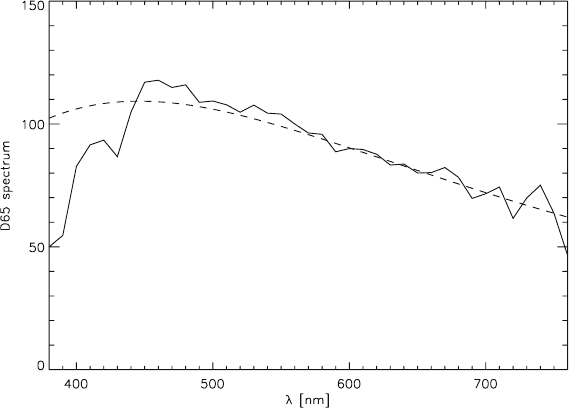
94 2 Foundations and Definitions
Fig. 2.7-3 Standard light D65 (dashed line shows black body radiation at 6,500 K)
and
R
sRGB
= [255 · R
+0.5] (2.7-16)
follow (analogously for G and B). [x] is the integer part of the real number x.
Secondly, the values R
sRGB
,G
sRGB
, B
sRGB
are transferred to the monitor. To
assess the colours visually the monitor must be situated in a dark room.
If an sRGB monitor is used together with a true colour sensor and D65 illumina-
tion and the sRGB values have been generated according to (2.7-14), (2.7-15) and
(2.7-16), the perceived colour impression should be nearly the same as if the illu-
minated object is being observed. This is the goal of the standardization. A parallel
process exists for printers but is not considered here.
Cameras are commercially available that have standard spectral value functions,
but most digital cameras have colour filters which deviate substantially from the
standard spectral value functions (Fig. 2.7-2). This is especially true in the case of
multispectral cameras such as Landsat-TM, SPOT and ADS40, in which relatively
narrow spectral channels are implemented which are optimised not for the gener-
ation of true colour images but for purposes of remote sensing. With such sensors
true colour can be created only approximately.
To discuss the problem in more detail, we consider a sensor with three narrow
band RGB channels at λR, λG, λB. If the scene is illuminated with monochromatic
light of wavelength λ which, for example, is positioned in the middle between λR
and λG, then the sensor cannot detect any light and the colour which corresponds
to the wavelength λ cannot be represented. The illuminated object is not seen by
2.8 Time Resolution and Related Properties 95
the sensor, but remains black. If the illumination is narrow-banded, therefore, over-
lapping spectral channels should be used. Airborne and spaceborne cameras for
photogrammetry and remote sensing do not have this problem: the illumination is
broad-banded and we can use narrow-band channels.
If a sensor has N spectral channels with the mid-wavelengths λ1, ...,λN, it gener-
ates N measurement values S1, ...,SN (for every pixel). For normal digital cameras
(red, green, and blue channel), N = 3. Multispectral sensors typically have N <10
channels, whereas hyperspectral sensors may have N > 100 spectral channels, so we
can generate three colour values X
, Y
, Z
according to
⎛
⎝
X
Y
Z
⎞
⎠
=
⎛
⎝
a
1,1
... a
1,N
a
2,1
... a
2,N
a
3,1
... a
3,N
⎞
⎠
·
⎛
⎜
⎜
⎜
⎜
⎝
S
1
...
...
...
S
N
⎞
⎟
⎟
⎟
⎟
⎠
. (2.7-17)
For certain classes of spectral data, this result may be adapted to the stan-
dard values X, Y, Z, which may be computed for these data according to (2.7-9).
This approach was successfully implemented, for example, for the ADS40, in
which the panchromatic channel added to the three colour channels R, G, B gives
N = 4 (Pomierski et al., 1998). The procedure may also be applied to ordinary dig-
ital cameras (N = 3; colour calibration) if good true colour capability is required.
This is especially useful if the output medium is calibrated too (for example, sRGB
standard for monitors).
2.8 Time Resolution and Related Properties
In this section, we introduce formulae and relations to enable the user of airborne
cameras to estimate the expected
• exposure times (integration times),
• data rates and volumes,
• camera viewing angles (FOV, IFOV) and
• stereo angles.
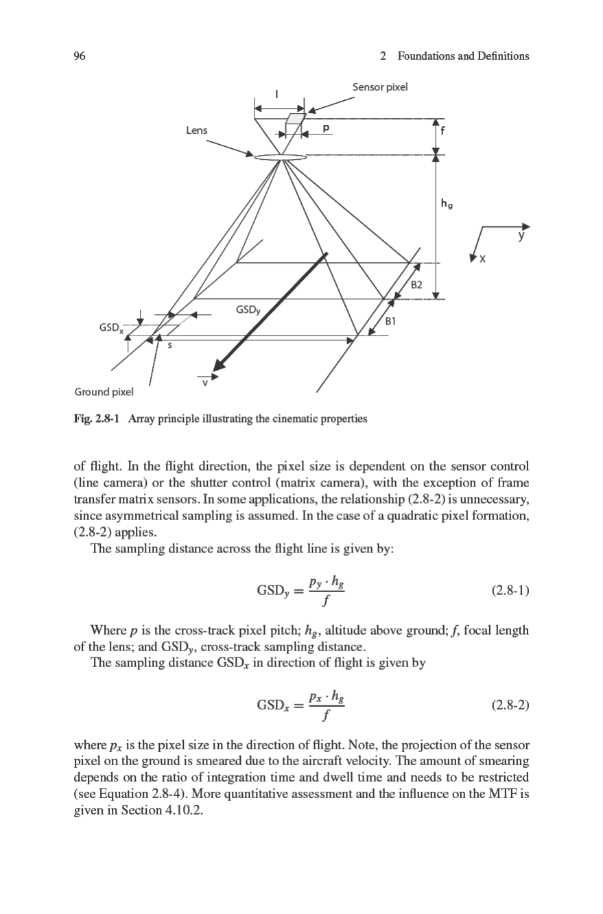
Figure 2.8-1 shows the array principle. It is assumed that the detector arrays (line
or matrix) have been placed in the image plane of the lens. It is further assumed that
the lens produces ideal geometric images without spherical aberration and, in the
case of sensors with spectral filters, without chromatic aberration.
As shown in Fig. 2.8-1, the derivation can be performed using the theorem on
intersecting lines and the ratio of the focal length of the lens f to the pixel size p
with reference to the scanning distance GSD
y
to flight altitude h
g
(see (2.8-1)). For
example, when h
g
= 1km,f = 62 mm and p = 6.5 μm, then GSD
y
= 10.5 cm.
The distance GSD
y
corresponds to the pixel size on the ground across the direction

2.8 Time Resolution and Related Properties 97
Flight speed v is an important variable in Fig. 2.8-1. As mentioned previously, in
photogrammetry one usually tries to obtain square images. Dwell time (maximum
cycle time for square sampling area) can be introduced for this approach. It is the
time needed to bridge the extension of the pixel projection in the direction of flight.
In line cameras, integration is started anew after each dwell time. In the case of a
matrix system, the start of a new integration is delayed according to the number of
pixels in the direction of flight and on the degree of overlap.
Geometric resolution in the case of integration times that correspond to the dwell
time does not change as a result of smearing of an entire pixel. Equation (2.8-3)
defines dwell time. This definition of the maximum possible cycle time (dwell time)
sets the maximum possible integration time of both line and matrix cameras:
t
dwell
=
GSD
x
v
(2.8-3)
The data rates D
line
and D
matrix
refer to a collection of k sensors, each with a
number N
P
of pixels. The effective data rates of matrix and line cameras also dif-
fer, since matrix cameras are typically used with a 60% overlap to generate stereo
images. The line camera data rate D
line
in pixels per second is given by:
D
line
=
k ·N
p
t
dwell
(2.8-4)
The stereo matrix camera data rate D
matrix
in pixels per second [results in 2.5
images per matrix frame] is:
D
matrix
=
k ·N
p
·2.5
t
dwell
(2.8-5)
The data volume is also dependent on radiometric resolution [bits] and on image
recording time [t
image
]. The number of bits required is typically filled up to the next
whole number byte limit. Thus, a 14-bit digital pixel value is represented by two
bytes [16 bits]. A conversion convention is required for this form of representation.
In most cases, the lowest-value bit of the 14-bit value is equated with the lowest-
value bit of the 16-bit value. The data volume Dv in bytes is defined by:
Dv[Byte] =
pixel
s
·t
image
·N
B
(2.8-6)
A finite number of pixels across the direction of flight is assumed for defining
the FOV (field of view). For example, in a line camera this would be the number
of pixels of the line sensor [Ns], and in the case of a matrix camera the cross-track
dimension of the matrix. As shown in Fig. 2.8-1, this dimension determines the
camera system’s swath. The triangular relationships required for (2.8-7) and (2.8-8)
can be readily understood if one imagines a plumb line from the nadir pixel along
the system’s optical axis:
FOV = 2 · arctan
0.5 · Ns · p
f
(2.8-7)

2.9 Comparison of Film and CCD 99
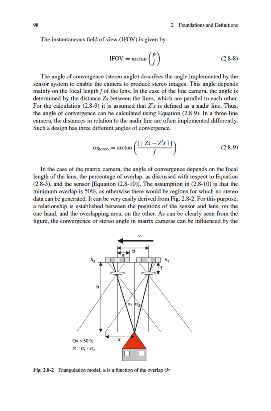
percentage of overlap. But on the other hand, it is influenced by the minimum time
required to read the matrix sensor. This imposes technological limits on the selection
of the percentage overlap.
α
Stereo
= arctan
x
h
+
a
f
·
(
1 − 2Ov
)
+arctan
a
f
−
x
h
(2.8-10)
An error parameter that directly influences the quality of stereo evaluation is the
stereo base to flight altitude ratio (B/h). It can be clearly seen in Fig. 2.8-2 that in
the case of matrix cameras, the base is dependent on the overlap set. Line cameras
have fixed angles of convergence, which can also be combined. This is has been
illustrated in Fig. 2.8-1. Bases B
1
and B
2
can be regarded separately or as a sum.
Thus, the general form (2.8-11) can be applied to both line and matrix cameras.
Consequently, the error parameter B/h can be regarded as
err = f
B
h
(2.8-11)
The differences between the bases of a line camera make it possible, with the aid
of an intelligent sensor control system, to include or exclude the lines with delay in
order to generate relevant stereo data.
2.9 Comparison of Film and CCD
Imaging with film and solid-state detectors (which are summarily called CCDs in the
following, although the radiometric quality of CMOS technology is almost equiva-
lent) is described by different statistical theories. These have consequences for the
characteristic curve and for different quality criteria, which can only be evaluated
together with the camera system. Hence, a comparison can refer either, as in this
section, to the fundamental physical boundaries, or to the practical consequences
for a special camera system.
Knowledge of the fundamentals of the photographic imaging process, CCD
technology and optical quantities is assumed here and can be drawn from, for
example, Sections 2.4 and 4.3 of this book, Schwidefski and Ackermann (1976),
Finsterwalder and Hofmann (1968), the Manual of Photogrammetry (McGlone
et al., 2004), and the Handbook of Optics (Bass et al., 1995).
2.9.1 Comparison of the Imaging Process and the Characteristic
Curve
Modern black and white film material features grain sizes in the range from 0.1 μm
to 3 μm – a typical value is 0.5 μm(Handbook of Optics, Section 20.2). Each grain
carries only 1-bit information (black/white) and it is necessary to invoke the concept
100 2 Foundations and Definitions
of an “equivalent pixel”, that is, a larger area, to allow the calculation of a gray value
as the proportion of black grains to the total number of grains. This equivalent pixel
size is defined, for example, by the MTF of the optics used, or by the pixel size of
the film scanning process and is in practice larger than 4 μm [typical values for film
scanning are 12–25 μm (McGlone et al., 2004, 402)].
A lower limit for the equivalent pixel is also the granularity of the film, which
originates in a statistical clustering of grains and leads to variations in the gray
value, even for homo-geneous illumination. In practice, at a transmission of 10%
(corresponding to a logarithmic density of D = 1), the granularity lies between
0.8 μm for fine-grain film and 1.1 μm for coarse-grain film (Finsterwalder and
Hofmann, 1968, 75).
Owing to the statistical distribution of the grains there is no aliasing in the
original film.
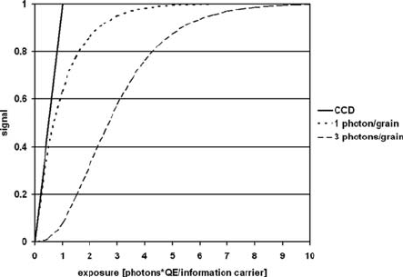
At least three photons are theoretically necessary to blacken a grain, but in prac-
tice the figure is ten or more (Dierickx, 1999). A Poisson distribution can therefore
be used to describe the likelihood that a grain is hit by a certain number of pho-
tons. The resulting cumulative distribution function for the event that three or more
photons strike the grain (the characteristic curve) is non-linear. For a three-photon
grain in the area of low exposure, it is initially proportional to the third power of
the number of striking photons and only then reaches the linear part of the function
(cf. Fig. 2.9-1). For a hypothetical one-photon grain, however, the density is pro-
portional to the number of photons from the beginning, in the case of low exposure
(Dierickx, 1999). The non-linear area at low exposure rates produces a gross fog
level followed by a low contrast area.
The roughly linear part of the function comprises about two logarithmic units or
7 bits and is described by the contrast factor γ (maximum gradient of the characteris-
tic curve), which for aerial films is in the range 0.9–1.5 (Finsterwalder and Hofmann,
Fig. 2.9-1 Signal as a function of normalised exposure for an ideal CCD and two different models
for film material