Saltzman B. (editor) Anomalous Atmospheric Flows and Blocking

Подождите немного. Документ загружается.

284

FREDERIKSEN

TABLE

PHASE

FREQUENCIES, GROWTH

RATES,

AND

PERIODS~

0.30486

0.25510

0.13536

0.20759

0.16698

0.35928

0.10662

0.42264

0.07 1627

0.16149

I2252

0.19731

0.08983

0.55

167

0.03059

0.09676

0.05758

0.24884

0.02386

I28288

0.08

154

0.0

109.7

91.8

48.7

74.7

60.1

129.3

38.4

152.2

25.8

58.1

44.

71.0

32.3

198.6

11.0

34.8

20.7

89.6

8.6

46.2

29.2

0.0

3.3

3.9

7.4

4.8

6.0

2.8

9.4

2.4

14.0

6.2

8.2

5.1

11.1

1.8

32.7

10.3

17.4

4.0

41.9

7.8

12.3

0.06796

0.06638

0.06246

0.06 195

0.06125

0.0599

0.05978

0.05499

0.05217

0.05216

0.05090

0.04498

0.04 128

0.0392

0.03593

0.03581

0.03454

0.03409

0.03358

0.03 I37

0.03

136

0.02725

0.4270

0.4171

0.3924

0.3892

0.3848

0.3764

0.3756

0.3455

0.3278

0.3277

0.3 I98

0.2826

0.2594

0.2464

0.2258

0.2250

0.2 170

0.2142

0.2 I09

0.1971

0.1970

0.1712

~~~

____

~ ~

____

~~ ~

Data

are

for

all

growing

modes,

from

the fastest to the

first nonpropagating

mode

for

Case

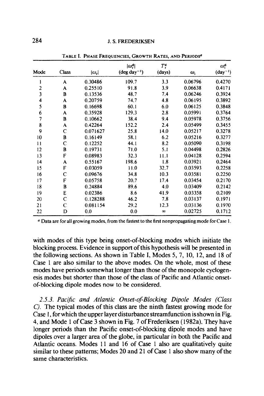
with modes of this type being onset-of-blocking modes which initiate the

blocking process. Evidence in support of this hypothesis will

presented in

the following sections.

shown in Table

Modes

10,

12, and 18 of

Case

are also similar to the above modes. On the whole, most of these

modes have periods somewhat longer than those of the monopole cyclogen-

esis modes but shorter than those of the class of Pacific and Atlantic onset-

of-blocking dipole modes now to

considered.

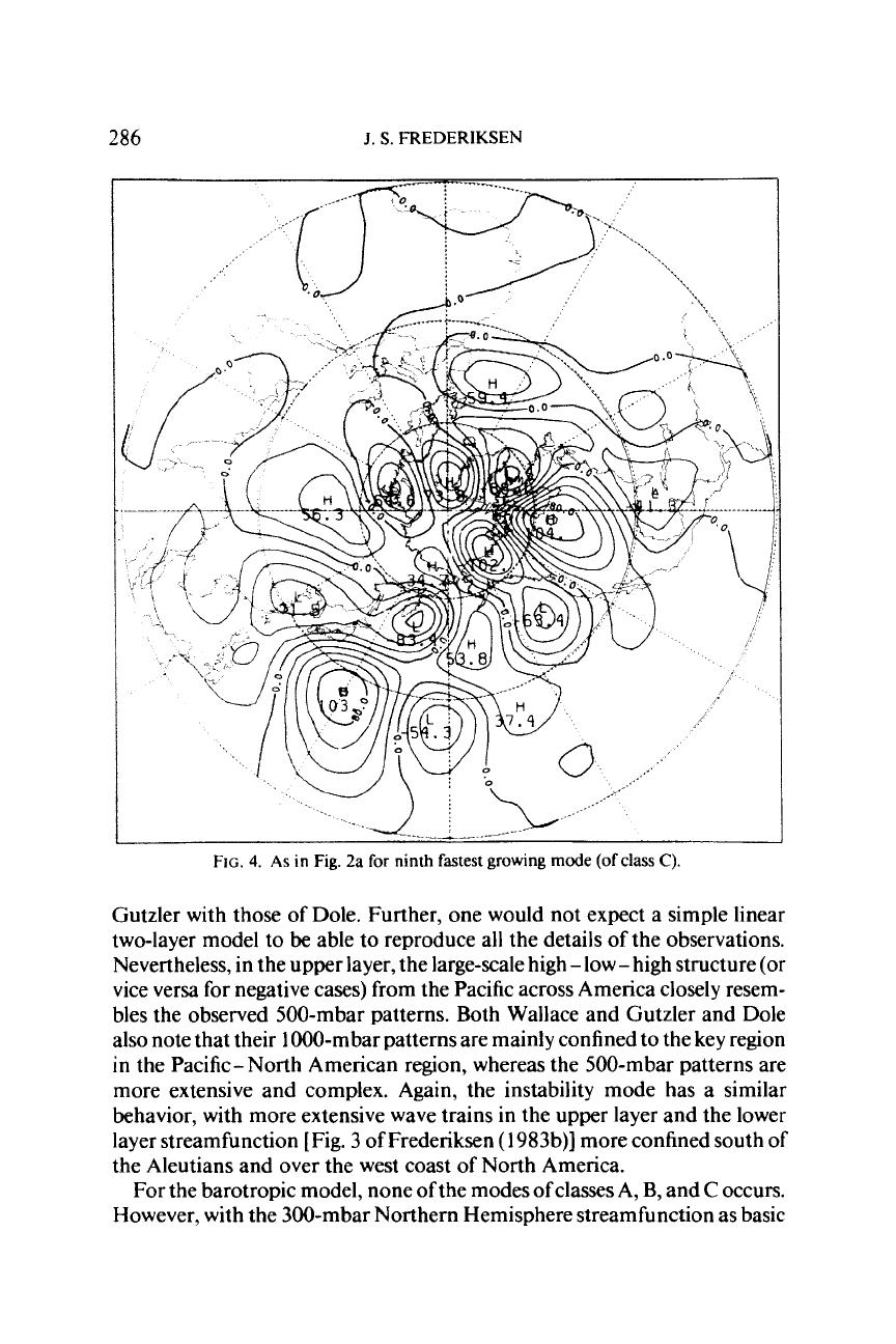
2.5.3.

Pacific

and

Atlantic

Onset-oJBlocking Dipole Modes

(Class

C).

The typical modes

this class are the ninth fastest growing mode for

Case

for which the upper layer disturbance streamfunction is shown in Fig.

and Mode

Case

shown in Fig.

of Frederiksen (1982a). They have

longer periods than the Pacific onset-of-blocking dipole modes and have

dipoles over a larger area

the

globe,

in particular in both the Pacific and

Atlantic oceans. Modes

1 1

and

Case

also

are qualitatively quite

similar to these patterns; Modes

and 2

Case

also

show many of the

same characteristics.

INSTABILITY THEORY AND NONLINEAR EVOLUTION

285

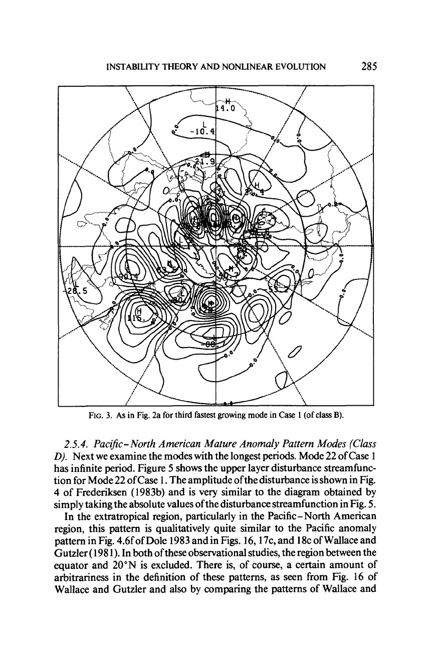
FIG.

Fig.

for

third

fastest

growing

mode

Case

(of

class

B).

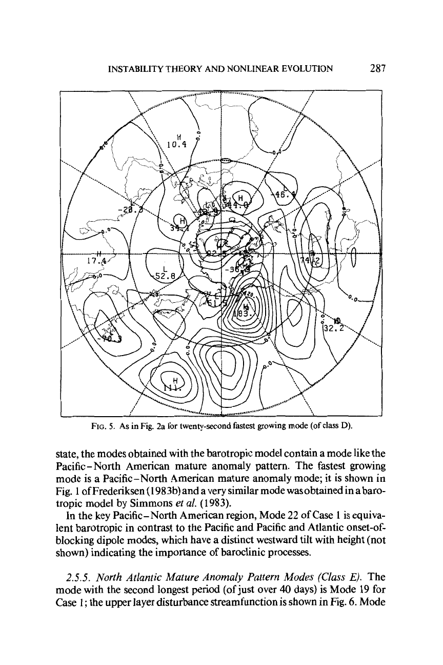
2.5.4.

PaciJic- North American Mature Anomaly Pattern Modes (Class

0).

Next we examine the modes with the longest periods. Mode

of Case

has infinite period. Figure

shows the upper layer disturbance streamfunc-

tion for Mode

of Case

The amplitude ofthe disturbance is shown in Fig.

Frederiksen (1983b) and is very similar to the diagram obtained by

simply taking the absolute values ofthe disturbance streamfunction in Fig.

In the extratropical region, particularly in the Pacific-North American

region, this pattern is qualitatively quite similar to the Pacific anomaly

pattern in Fig. 4.6f of Dole 1983 and in Figs. 16,17c, and I8c of Wallace and

Gutzler

(

198

I).

In both of these observational studies, the region between the

equator and

20"N

is excluded. There is, of course, a certain amount

arbitrariness in the definition of these patterns, as seen from Fig.

Wallace and Gutzler and also by comparing the patterns of Wallace and

286

FREDERIKSEN

FIG.

Fig.

for

ninth

fastest

growing

mode

(of

class

C).

Gutzler with those of Dole. Further, one would not expect a simple linear

two-layer model to

able to reproduce all the details of the observations.

Nevertheless, in the upper layer, the large-scale high -low

high structure (or

vice versa for negative cases) from the Pacific across America closely resem-

bles the observed 500-mbar patterns. Both Wallace and Gutzler and Dole

also note that their 1000-mbar patterns are mainly confined to the key region

the Pacific-North American region, whereas the 500-mbar patterns are

more extensive and complex. Again, the instability mode has a similar

behavior, with more extensive wave trains in the upper layer and the lower

layer streamfunction [Fig.

of Frederiksen

(

1983b)l more confined south of

the Aleutians and over the west coast of North America.

For the barotropic model, none

the modes of classes A,

and

occurs.

However, with the 300-mbar Northern Hemisphere streamfunction as basic

287

INSTABILITY THEORY AND NONLINEAR EVOLUTION

FIG.

Fig.

for

twenty-second fastest growing mode

(of

class

D).

state, the modes obtained with the barotropic model contain a mode like the

Pacific- North American mature anomaly pattern. The fastest growing

mode is a Pacific-North American mature anomaly mode; it is shown in

Fig.

of Frederiksen

983b) and a very similar mode was obtained in a baro-

tropic model by Simmons

et al.

(

1983).

In the key Pacific-North American region, Mode

of Case

is equiva-

lent barotropic in contrast to the Pacific and Pacific and Atlantic onset-of-

blocking dipole modes, which have a distinct westward tilt with height (not

shown) indicating the importance of baroclinic processes.

2.5.5.

North Atlantic Mature Anomaly Pattern Modes (Class

E).

The

mode with the second longest period (of just over

days) is Mode 19 for

Case

;

the upper layer disturbance streamfunction is shown in Fig.

Mode

288

FREDERIKSEN

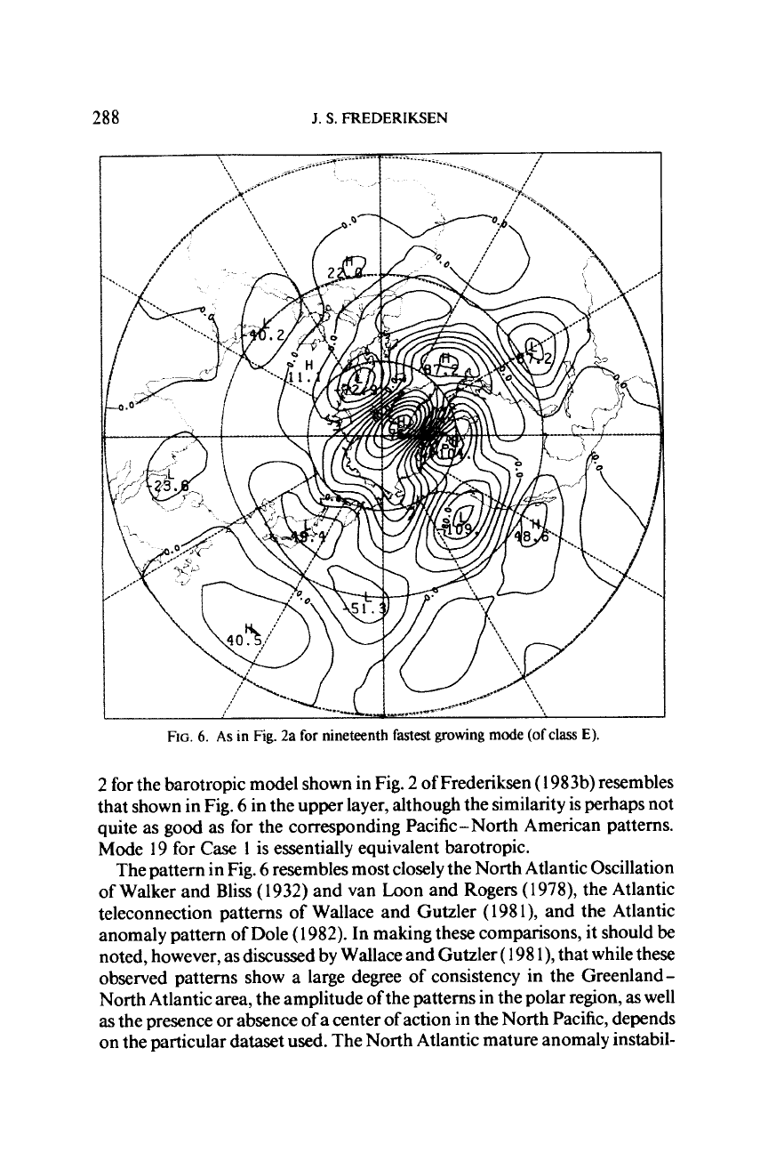
FIG.

Fig.

for

nineteenth

fastest

growing mode

(of

class

E).

for the barotropic model shown in Fig.

of Frederiksen

(

1983b)

resembles

that shown in

Fig.

in the upper layer, although the similarity is perhaps not

quite as

good

as for the corresponding Pacific

North American patterns.

Mode 19 for

Case

essentially equivalent barotropic.

The pattern in Fig.

resembles most closely the North Atlantic Oscillation

of Walker and Bliss

(1932)

and van Loon and Rogers (1978), the Atlantic

teleconnection patterns

Wallace and Gutzler

(198

l),

and the Atlantic

anomaly pattern of Dole

(

1982). In making these comparisons, it should be

noted, however, as discussed by Wallace and Gutzler

(

198 l),

that while these

observed patterns show a large degree of consistency in the Greenland-

North Atlantic area, the amplitude

the patterns in the polar region,

well

the presence or absence

a center of action in the North Pacific, depends

on the particular dataset

used.

The North Atlantic mature anomaly instabil-

INSTABILITY

THEORY

AND

NONLINEAR

EVOLUTION

289

ity mode appears to bear closest resemblance to the sea level pressure anom-

aly pattern in Fig.

of van Loon and Rogers (1978).

2.5.6.

IntermediateModes (Class

F).

Among the modes in Table

there

is also a group whose properties, in qualitative terms, are intermediate be-

tween the onset-of-blocking dipole modes and the mature anomaly pattern

modes discussed above. Mode 15

Case

has the third largest period

(of

30 days); Fig. 6

Frederiksen (1983b) shows the disturbance stream-

function. As seen there, this mode appears to have characteristics of both of

the major mature anomaly modes previously discussed. However, the scale

of the centers making up the mode appears on the whole to be smaller.

Modes 17 and

3 of Case

have similar structures and periods of

7.4 and

1.1

days, respectively; Fig. 7 of Frederiksen (1983b) shows the perturbation

streamfunction for Mode 17. These modes have properties and, in particu-

lar, scales intermediate between the mature anomaly pattern modes and the

Pacific and Atlantic onset-of-blocking modes.

TIME EVOLUTION

OBSERVED MATURE

ANOMALIES

At the time of the study of Frederiksen

(

1982a), there appeared to be no

systematic statistical studies on the observed time evolution of mature

anomalies such

blocks. Nevertheless, it seemed reasonable that the slower

propagating modes with dipoles in the Pacific and Atlantic regions, called

class

and C modes here, would initiate the process of the formation of

mature anomalies such as blocks further downstream.

The thesis of Dole (1982), parts

which have been published in Dole

(1983) and also in this volume, provided important insights into many

aspects

observed mature anomalies, including their time evolution. Here

we shall relate some

the instability solutions of Section 2 to Dole’s obser-

vations.

In our discussion

Dole’s studies, we shall concentrate on anomalies

corresponding to the Pacific-North American pattern, since this is the case

for which he gives the most extensive analysis. Similar results also hold for

the North Atlantic (and northern Soviet Union) anomalies, which he also

treats in lesser detail. Dole finds in his studies not only positive anomalies in

the key region corresponding to blocking, but also negative anomalies. He

notes that the two extreme stages of the index cycle (Namias, 1950) appear in

his analyses

opposite phases of

single basic anomaly pattern, with high

zonal index corresponding to negative anomaly and low zonal index corre-

sponding to positive anomaly, such as caused by blocking.

Figure 4.6

Dole (1983) shows the time evolution of composite analyses

290

FREDERIKSEN

low-pass-filtered positive anomaly cases at

500

mbar in the Pacific. The

sequence starts

days before (on day

-4)

the appearance (on day

the essentially stationary large-scale positive anomaly in the key region in the

north central Pacific and finishes

days thereafter. The corresponding se-

quences for unfiltered anomalies between days -3 and

are shown in Fig.

4.7 of Dole (1983). For the period leading up to the appearance of the

positive anomaly in the key region, referred to in Frederiksen

982a) as the

onset-of-blocking period, Dole notes that the “sequence

of development

suggests that the initial rapid growth of the main centre is primarily asso-

ciated with the propagating intensifying disturbance which originates in

mid-latitudes near Japan.” He also notes that “this disturbance continues to

intensify as it becomes quasi-stationary over the key region.” The dipole

wave train that appears in Fig.

4.7

of Dole (1983) at day -3 is qualitatively

very similar to that in our Fig. 3 and as well to that in Fig. 6a of Frederiksen

(

1982a).

Further evidence that modes

class

are involved in the initial period

may

obtained from Fig.

5.10

Dole (1982), which shows longitude-

pressure cross sections at

45”

and 20”N of the unfiltered Pacific composite

anomalies at I-day intervals between days -3 and

The dipole nature of the developing anomaly is clearly evident particu-

larly at day -3, and the zonal scale of the anomaly at day -3 is practically

the same as shown in Fig.

of Frederiksen (1982a) and in our Fig. 3. The

developing anomaly has a definite westward tilt with height, as do the class

modes. Dole notes: “This feature has pronounced westward tilts with height

during this period, suggesting that a substantial baroclinic contribution is

involved in its amplification.”

Following day

the development of the 500-mbar height anomaly

shown in Fig.

Id-

of Dole

(

I982), with the anomalies being largely equiv-

alent barotropic during this

period.

Intensification

the centers occur with

little phase propagation and by day

and especially at day

the Pacific-

North American pattern is established.

The above observational and theoretical results suggest that the develop-

ment of mature anomalies such as blocks may be thought of as approxi-

mately consisting of two stages, which, for the Pacific- North American

pattern, are as follows:

rapidly growing and relatively rapidly eastward-propagating dipole

(class

disturbance which tilts westward with height forms in the Pacific

Ocean

East

Asia region through the combined baroclinic

barotropic in-

stability

the three-dimensional basic state.

the disturbance grows, the

regions of largest amplitude propagate into the central Pacific and the distur-

bance increases its zonal scale, becoming quasi-stationary and essentially

INSTABILITY

THEORY

AND NONLINEAR

EVOLUTION

equivalent barotropic through the operation of nonlinear effects. At this

stage the mode has a structure reminiscent of class

modes.

The (nonlinear analog of

class

mode amplifies without phase

propagation and through the operation of largely equivalent barotropic ef-

fects to form the large-amplitude mature Pacific- North American anomaly

pattern.

We have concentrated in this section on the composite results of Dole

(

1983), which present a very clear-cut example of the change in the horizon-

tal and vertical structures of the anomaly pattern, starting upstream of the

key region with the formation of westward-tilting smaller scale dipole distur-

bances. The importance of transients in the development of blocks has also

been pointed out by many other authors, e.g., Lejenas (1 977), Green

(

1977),

Austin

(

1980), Youngblutt and Sasamori (1 980), Tucker

(

1979), Illari and

Marshall (1983), Colucci (1982), Hansen and Chen (1982), and Shutts

(1983). Hansen and Chen, in particular, note that in their observational

studies of blocking, intense upstream cyclogenesis preceded the growth of

the blocking ridge. Further, “the nonlinear transfer of kinetic energy from

baroclinically active cyclone-scale waves to the planetary-scale waves pro-

vided the major source of kinetic energy for the block.” Lejenas

(

1977) notes

the importance of the combination of barotropic and baroclinic instability

during the formation

blocks. Barnett (1984), in an observational study,

also

finds support for instability normal modes playing important roles in

the generation of anomaly patterns.

For the Southern Hemisphere, Frederiksen (1984, 1985) has carried out

three-dimensional instability studies for climatological flows and for synop-

tic flows leading to the formation

blocks in the Australian

New Zealand

area, as well as cyclogenesis in a number ofregions. Instability theory appears

to be able to pick out many of the important developments. In particular,

dipole instability modes are produced in

slightly upstream of the blocking

region. Lejenas (1 984), in an observational study

Southern Hemisphere

blocking, also finds support for dipole instability modes being responsible

for the majority of blocking episodes while the additional influence of forc-

ing controls the duration.

4. NONLINEAR SIMULATION

Next, we relate the results of numerical simulations of evolving baroclinic

waves to the properties of the instability solutions and to observations of

developing anomalies. We shall primarily consider a study by Frederiksen

and Pun

(

1985) of nonlinear baroclinic waves growing on an initial three-di-

292

FREDERIKSEN

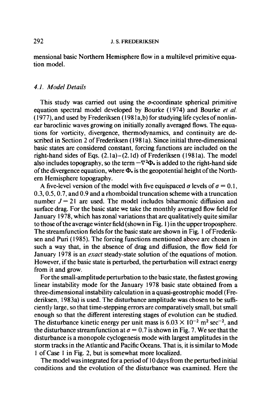
mensional basic Northern Hemisphere flow in a multilevel primitive equa-

tion model.

4.1.

Model Details

This study was camed out using the a-coordinate spherical primitive

equation spectral model developed by Bourke (1974) and Bourke

al.

(1977), and used by Frederiksen

(

198

la,b) for studying life cycles of nonlin-

ear baroclinic waves growing on initially zonally averaged flows. The equa-

tions for vorticity, divergence, thermodynamics, and continuity are de-

scribed in Section 2 of Frederiksen

(

198

a). Since initial three-dimensional

basic states are considered constant, forcing functions are included on the

right-hand sides of

Eqs.

(2.la)-(2.ld) of Frederiksen (1981a). The model

also includes topography,

the term

-OW.

is added to the right-hand side

of the divergence equation, where

is the geopotential height ofthe North-

Hemisphere topography.

A five-level version of the model with five equispaced

levels of

0.1,

0.3,0.5,0.7, and 0.9 and a rhomboidal truncation scheme with

truncation

number

21 are used. The model includes biharmonic diffusion and

surface drag. For the basic state we take the monthly averaged flow field for

January 1978, which has zonal variations that are qualitatively quite similar

to those of the average winter field(shown in Fig.

in the upper troposphere.

The streamfunction fields for the basic state are shown in Fig.

of Frederik-

sen and Pun

(

1985). The forcing functions mentioned above are chosen in

such a way that, in the absence of drag and diffusion, the flow field for

January 1978 is an

exact

steady-state solution of the equations of motion.

However, if the basic state is perturbed, the perturbation will extract energy

from it and grow.

For the small-amplitude perturbation to the basic state, the fastest growing

linear instability mode for the January 1978 basic state obtained from a

three-dimensional instability calculation in a quasi-geostrophic model (Fre-

deriksen, 1983a) is used. The disturbance amplitude was chosen to

suffi-

ciently large,

that time-stepping errors are comparatively small, but small

enough

that the different interesting stages of evolution can be studied.

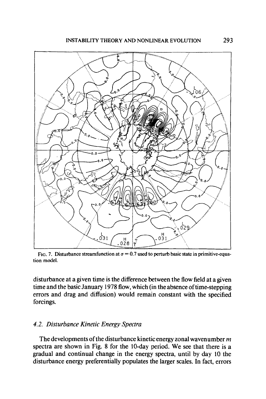
The disturbance kinetic energy per unit mass is

6.03

m2 sec2, and

the disturbance streamfunction at

0.7 is shown in Fig. 7. We see that the

disturbance is a monopole cyclogenesis mode with largest amplitudes in the

storm tracks in the Atlantic and Pacific Oceans. That is, it is similar to Mode

Case

in Fig. 2, but

somewhat more localized.

The model was integrated for a

period

days from the perturbed initial

conditions and the evolution of the disturbance was examined. Here the

INSTABILITY THEORY AND NONLINEAR EVOLUTION

293

FIG.

Disturbance streamfunction at

0.7

used to perturb basic state in primitive-equa-

tion model.

disturbance at a given time is the difference between the flow field at a given

time and the basic January 1978 flow, which (in the absence of time-stepping

errors and drag and diffusion) would remain constant with the specified

forcings.

4.2.

Disturbance Kinetic Energy Spectra

The developments of the disturbance kinetic energy zonal wavenumber

spectra are shown in Fig.

for the 10-day period. We see that there is a

gradual and continual change in the energy spectra, until by day

the

disturbance energy preferentially populates the larger scales. In fact, errors