Roy K.K. Potential theory in applied geophysics

Подождите немного. Документ загружается.

13.11 Sphere in the Field of a Vertically Oscillating Magnetic Dipole 439

It is assumed that µ = µ

Since

′

3/2

(α)=I

1/2

(α) −

2α

3/2

(α)

1/2

(α)=



πα



1/2

sin hα

and

3/2

(α)=



πα



1/2



cosh α −

sin hα



canbewrittenintheform

= −

.Ha

asinhα − (2γ +1)



cosh α −

sin hα



α sin hα +(γ − 1)



cosh α −

sinh α



= −

− (2γ +1)(α coth α −1)

+(γ −1) (α

coth α −1)

= −

S. (13.418)

Hence



Hr sin θ −

S sin θ (13.419)



= H cos θ − H

S cos θ (13.420)

(normal ﬁeld) ↓ (perturbation ﬁeld) ↓



= −H sin θ −

.S sin θ (13.421)

(normal ﬁeld) (perturbation ﬁeld)

If we take M = −

S, the radial and angular components are



Mcosθ



Msinθ

(13.422)

The eﬀect of a sphere is as if a dipole is oriented along the Z-axis and it is

placed at the centre. We can express the vertical and horizontal components



cos θ −



sin θ (13.423)

=H−



−

(13.424)

440 13 Electromagnetic Wave Propagation

where

(13.425)

and



sin θ +



cos θ = −

3hy

. (13.426)

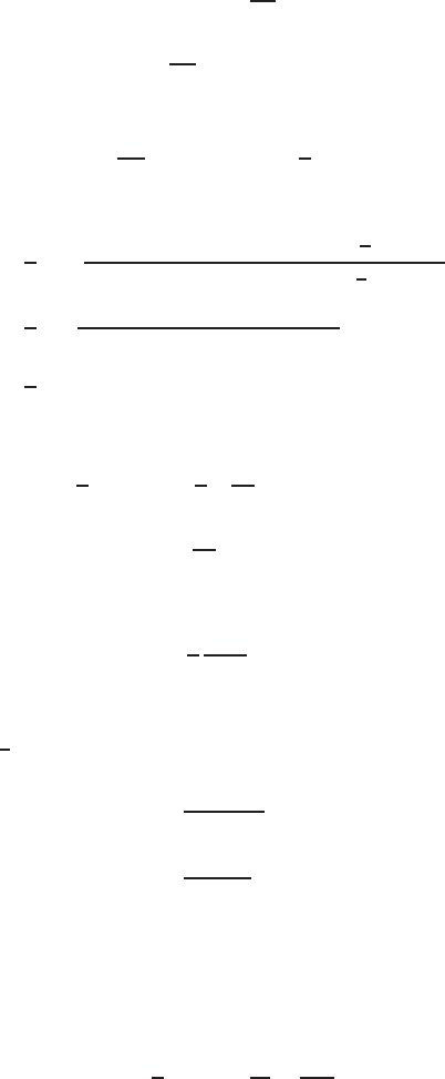
Here the vertical ﬁeld is only the normal component and it will be maximum

at y = 0 and the horizontal component will be maximum i.e.,



∂H



will b e

maximum at y = ±

√

(Fig. 13.18). Hence the anomaly ﬁeld depends upon

the S and geometry of the body.

HereS=M+iNwhereMandNarerespectively the in phase and quadra-

ture components.

Now for smaller values of ‘α’

S=−

3α (coth α −1) −α

(13.427)

=1+

−

3cothα

. (13.428)

Since

coth α =1+

−

+ ....., (13.429)

Fig. 13.18. Variation of horizontal and vertical magnetic ﬁeld over a buried sphere-

ical inhomogenities

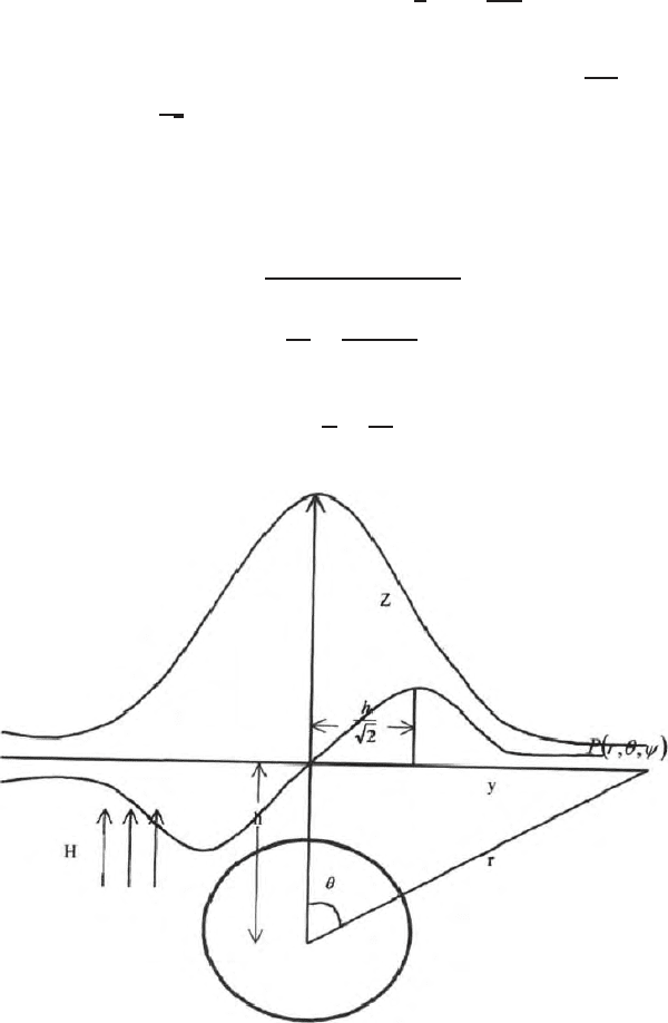
13.12 Principle of Electrodynamic Similitude 441

Fig. 13.19. A conducting plate of radius a and thickness t

the approximate value of S

S ≈

ωµσ.

For a spherical body, the multiplication factor to α

ωµσ is

instead of

the case of an inﬁnitely long cylinder. For a circular plate of ﬁnite diameter

and thickness the response factor is

at ωµσ whereaistheradiusofthe

plate and t is the thickness (Fig. 13.19).

The frequency response for all bodies (conductive or resistive) can be writ-

ten as |F| =kL

ωµσ where k is the multiplication factor.

13.12 Principle of Electrodynamic Similitude

From Maxwell equations cur l



E = −μ

∂



∂t

,andcurl



H = σ



E+ ∈

∂E

∂t

div







=0,div



∈





= 0 where there is no source in the region. Let

and t

represent the unit of length and time. ∈

,μ

and h

are the cor-

responding units of electrical permittivity, magnetic permeability, electric ﬁeld

and magnetic ﬁeld. We can then write l = l

′

,t= t

′

,E= e

′

andH =

′

. Curl has the dimension of 1/l ength. We can then write from Maxwell’s

ﬁrst equation.

.Curl

′

= −

.μ

′

(13.430)

Here curl is a pure number.

From Maxwell’s second equation we get,

.Curl

′

= σ

′

∈

′

∂E

′

∂t

. (13.431)

we can write from (13.430) and (13.431)

.Curl

′

= −

.μ

′

∂H

′

∂t

′

(13.432)

and

curl H

′

= −

.σ

′

∈

. ∈

′

∂E

′

∂t

. (13.433)

442 13 Electromagnetic Wave Propagation

From t hese two equations, we can write

. = constant k

(13.434)

. = constant = k

and

∈

= constant = k

. (13.435)

Since the Maxwell’s equations are valid, these factors will be constants. From

these three equations, we can write

∈

(13.436)

∈

(13.437)

Thus

. = constant and

∈

= constant.

From t hese two equations, we can write

= constant (13.438)

and

∈

= constant (13.439)

These are two basic equations of the electrodynamics similitude. Usually the

displacement current will be signiﬁcant when the frequency is of the order of

. That is in the megahertz range frequency, both the equations must be

satisﬁed for any kind of model simulation. For geophysics, where the operating

frequency is in the audio frequency range, the displacement current is negli -

gible and only one equations must be satisﬁed for simulation of models i.e.,

= constant. Thus l

wμσ is the electromagnetic response parameter

and is used in geophysical exploration. If M stands for the model and F stands

for the ﬁelds data, then

= μ

(13.440)

where μ, σ, w , and L are respectively the magnetic permea b ility, electrical

conductivity, angular frequency and linear dimension of the model. When we

simulate the electgromagnetic model for non magnetic materials,

= μ

and the (13.440) reduces to

13.12 Principle of Electrodynamic Similitude 443

= L

(13.441)

Once we set up the model for a particular s et of L

ωμσ = constant, we

can utilise the response function by suitably multiplying it by a constant.

In otherwords, we know responses due to a (i) sphere



wμσ



(ii) cylin-

der



ωμσ



and (iii) plate



atwμσ



, we have to ﬁnd out the suitable

multiplication factor for b odies of other geometrical shapes for the relation

wμσ.

Green’s Function

In this chapter we brieﬂy discussed about some of the basic natures of Green’s

function. It is a mathematical to ol having multifaceted application in vari-

ous branches of applied mathematics and mathematical physics. Some of the

properties and applications of Green’s function in potential theory a re given.

Dyadics and dyadic Green’s functions are deﬁned. The nature of scalar and

tensor Green’s function are shown. Application of Green’s function in math-

ematical modeling is given in Chap. 15.

14.1 Introducti on

Green’s function is a mathematical tool used to solve potential and nonpoten-

tial boundary value problems in scalar and vector potential ﬁeld domain. It

can represent a potential function which is harmonic and regular maintaining

some diﬀerences in their properties with potential function at the boundaries.

In the vector potential ﬁeld domain it can represent a ﬁeld or a vector poten-

tial. Green function can be a tensor in the vector p otential ﬁeld domain and

both scalar and tensor Green’s function can b e the kernel function in the Fred-

hom’s or Volterra,s integral equations. In the presence of a boundary surface

nearby, image of a source appears in the Green function’s formula. Green’s

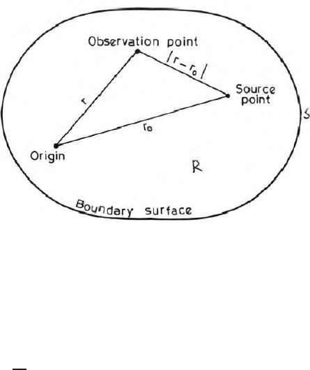
functions are always associated with two points say G(r, r

) where r and r

are respectively the distances of the o bservation point and source po int from

an assumed origin in the space domain (Fig. 14.1).

These points may be within a domain R or one of the points may be

within a domain and the other point may be on the surface S which binds

the domain. This surface may be at ﬁnite distance from the source or it may

be at inﬁnite distance. So Green’s functions are generally associated with the

boundary conditions and/or initial conditions. It is used as a mathematical

tool for solution of elliptic, parabolic and hyperbolic diﬀerential equations

(see Chap. 2) with homogeneous and inhomogeneous boundary conditions.

446 14 Green’s Function

Fig. 14.1. A green’s function domain with source point, observation point, boundary

surface and origin

It is often used in some cases for solution of Poisson and Laplace equa-

tion with homogeneous and inhomogeneous Dirichlet, Neumann and mixed

(Robin or Cauchy) boundary conditions. Once Green’s function is evalu-

ated for homogeneous equation (say Laplace equation) with homogeneous



say φ =0or

∂φ

∂n

= 0 on the boundary



boundary conditions it can be used

for inhomogeneous equations with inhomogeneous boundary conditions in

some cases.

The form, application and method of determining Green’s function vary

from problem to problem in time and space domain. It depends upon the ﬁeld

where it is applied as well as on the guiding equation. It vanishes on the su r-

face of a bounded region. It can represent a potential at a point due to an unit

source. It can reduce the unknowns to be deter mined in a potential problem

Green’s function is symmetric and the principle of reciprocity is valid. Some

of the discontinuities in a potential function at boundaries are removed in

Green’s function domain. Green’s function also can have discontinuity on the

boundary. Green’s function can be used as a mathematical tool for solution of

problems related to heat conduction, electromagnetic wave propagation, em

transients initial value problems, impulse response problems etc. The proce-

dural details for evaluation of the Green’s function diﬀer in diﬀerent topics

of mathematical physics. So far as geophysics is concerned the major appli-

cation of Green’s function lies in solution of boundary value problems using

Integral Equation method where non dyadic form appears in direct current

ﬂowﬁeldoranyotherscalarpotentialﬁeld and dyadic form appears in elec-

tromagnetic ﬁeld.. For solution of Laplace’s equation, we have other options

like series solution of harmonic function, method of separation of variable ,

conformal transformation etc. We need not go for Greens function for all types

of problems specially where evaluation of Green’s function may invite tougher

14.2 Delta Function 447

mathematics. For time varying EM ﬁelds, the Green’s function appear in the

form of a dyadic function generally since the scalar is replaced by a vector and

dot product appears in place of algebraic product. Dot product with a vector

source appears only if G, the Green’s function is in the form of a dyadic. Since

in vector potential domain both the ﬁeld and the potential are vectors and

Green,s function can represent both the ﬁelds and vector potentials. In vector

potential domain both scalar and tensor Green’s functions co exist. Green’s

theorem has a major role in evaluating Green’s function in potential theory.

Vector Green’s function and tensor algebra have contribution towards der iv-

ing dyadic Green’s function obtained from Helmholtz electromagnetic wave

equation. It is dyadic for a vector source and nondyadic for a scalar source.

The way so me similarities exist in operations between a matrix inverse

and an operator inverse, an identity matrix and an idem factor or an iden-

tity operator in operator domain, some such similarities do exist between a

nine component second order tensor and a dyadic. A few simple examples of

determining Green’s function are given.

This topic is brieﬂy introduced in this chapter. Further details are avail-

able in Lanczos (1941, 1997), Morse and Feshbach (1953), Blakely (1996),

Tai (1971), Stackgold (1968, 1979), Roach (1970), Sneider (2001), Macmil-

lan (1958), Sobolev (1981), Ramsay (1959), Barton(1989), Van Bladel (1968),

Hohmann (1971, 1975, 1983, 1988).

14.2 Delta Function

Dirac delta function was introduced by Paul Dirac. It states that a function

‘r’ is assumed to vanish everywhere outside the point at r = r

.Atthepoint

r=r

, the value of the function δ(x, r) becomes in ﬁnitely high such that the

total area or volume under the curve is unity. It can be expressed as

∫ δ(r −r

)dr=1. (14.1)

One can write

=1fori=j

=0fori= j (14.2)

where δ

are the values of an identity matrix and it is known as Kronecker

delta, i.e., I

= δ

, where I is the identity matrix. For a multidimensional

space, we have

δ(r − r

)=δ(x −x

) δ(y − y

) δ(z − z

) (14.3)

where x, y, z are the three coordinates in an Euclidian space and the co ordi-

nates of r and r

are respectively (x, y, z) and (x

, y

, z

In the integral form, we have



δ(r −r

)f(r)dv =



δ(x − x

)δ(y − y

)δ(z −z

)f(x

)dxdydz (14.4)

448 14 Green’s Function

14.3 Operators

Solution of a boundary value problem is an important area in mathemat-

ical physics. It initiates the mathematical formulation of forward problems

which is a basic ingredient for solving an inverse problem needed for inter-

pretation of geophysical data. Many of the forward problems are based on

elliptic, parabolic a nd hyperbo li c type of diﬀerential equations. In some cases

these equations can be ordinary diﬀerential equations. These equations can

be written as

LΦ = f (14.5)

where L is the operator. It can be a linear or nonlinear diﬀerential opera-

tor. Φ is the unknown function to be determined and f is a known function.

Equation (14.5) can be a ﬁrst, second or higher order ordinary or partial

diﬀerential homogeneous or inhomogeneous equations with homogeneous or

inhomogeneous boundary conditions. The diﬀerential operators are

(14.6)

(14.7)

∂

∂x

∂

∂y

∂

∂z

(14.8)

Equation (14.8) is also known as Laplace or Poisson operator for second order

partial diﬀerential equations and is denoted by ∇

and ∆. Using the same

operator we can write Laplace, Poisson and Helmholtz equations as

Lφ =∆φ = ∇

φ = 0 (14.9)

Lφ =∆φ = ∇

φ = f (14.10)

Lφ =∆φ = ∇



H=γ

H (14.11)

One of the methods for solving the partial diﬀerential equation is to go for

searching an inverse operator L

−1

where L

−1

L=LL

−1

=IwhereIisthe

identity operator. Since L is the diﬀerential op erator, L

−1

is termed as an

inverse integral operator. Nature of these integral operators takes the form of

Fredhom or Volterra’s integral equation. The kernel of this integral is termed

as the Green’s function for the operator L. Assuming L to be a linear o r linear

diﬀerential operator, we get

−1

φ(x) =



(x, x

)φ(x

)dx

. (14.12)

From the relation L

−1

L=LL

−1

=I,wecanwrite

φ(x) = Iφ(x) = LL

−1

φ(x) = L ∫ G

(x, x

) φ(x

)dx

⇒∫G(x, x

) φ(x

)dx

(14.13)

where LG

(x, x

)=G(x, x

)