Roy K.K. Potential theory in applied geophysics
Подождите немного. Документ загружается.


13.10 Electromagnetic Induction due to an Infinite Cylinder 429
H=curl
A (13.329)
⇒ curl curl
A =(σ + iω ∈)
E (13.330)
⇒ grad div
A −∇
2
A =(σ + iω ∈)
E (13.331)
⇒ grad div
A − iωμ (σ + iω ∈)
A =(σ + iω ∈)
E (13.332)
⇒
E = −iωμ
A +
1
σ + iω ∈
grad div
A. (13.333)
We can write the magnetic field comp onents from (13.329) as
H
r
=
1
r
∂
A
z
∂ψ
−
∂
A
ψ
∂z
(13.334)
Hψ =
∂
A
r
∂z
−
∂
A
z
∂r
(13.335)
H
z
=
1
r
∂
∂r
r
A
ψ
−
1
r
∂A
r
∂ψ
. (13.336)
Since
∂
∂z
=0andA
ψ
=0andA
r
=0,weget
H
r
=
1
r
∂
A
z
∂ψ
(13.337)
H
ψ
= −
∂
A
z
∂r
(13.338)
H
z
=0. (13.339)
The wave equation can be written in the form
∂
2
A
z
∂r
2
+
1
r
∂
A
z
∂r
+
1
r
2
∂
2
A
z
∂ψ
2
= γ
2
A
z
which is independent of the variation along the z-direction.
Applying the method of separation of variables we have
A =RΨ (13.340)
d
2
Ψ
dψ
2
+ n
2
Ψ =0 (13.341)
and
d
2
R
dr
2
+
1
r
dR
dr
−
γ
2
+
n
2
r
2
R=0. (13.342)
The solutions are
(i) cos mψ, sin mψ
and

430 13 Electromagnetic Wave Propagation
(ii) I
n
(γr), K
n
(γr). (13.343)
The vector potentials outside and inside the body are given by
A
0
=Hrsinψ +
(c
n
cos nψ +d
n
sin nψ)K
n
(γr) (13.344)
and
A
i
=
(f
n
cos nψ +g
n
sin nψ)I
n
(γr). (13.345)
At the boundary of the cylinder i.e., at
r=a,
Hψ
0
=
Hψ
1
(13.346)
E
z
0
=
E
z
1
(13.347)
∂A
0
∂r
=
∂A
1
∂r
(13.348)
µ
0
A
0
= µ
1
A
1
. (13.349)
Applying the first boundary condition, we get
µ
0
Ha sin φ + µ
0
(c
n
cos nψ +d
n
sin nψ)K
n
(γ
0
a)
= µ
1
(f
n
cos nψ +g
n
sin nψ)I
n
(γ
1
a). (13.350)
Equating the coefficients of sines and cosines we get,
µ
0
C
n
K
n
(γ
0
a) = µ
1
f
n
I
n
(γ, a). (13.351)
Since the source field does not contain any cosine term, the secondary field
also should not contain any cosine terms. Therefore
c
n
=f
n
=0. (13.352)
Similarly
d
n
=g
n
= 0 except for n = 1 (13.353)
and
µ
0
Ha + µ
0
d
1
K
1
(γ
0
a) = µ
1
g
1
I
1
(γ
1
a) . (13.354)
From the second boundary condition
H + d
1
γ
0
K
′
1
(γ
0
a)=g
1
γ
1
I
1
(γ
1
a) . (13.355)
From t hese two equations
d
1
= H
μ
1
I
1
(γ
1
a) − μ
0
γ
0
aI
1
(γ
0
a)
μ
0
γ
1
k
1
(γ
0
a) I
1
(γ
1
a) −μ
1
γ
0
I
1
(γ
1
a)(γ
0
a)
. (13.356)
The vector potential outside the cylinder is given by
13.10 Electromagnetic Induction due to an Infinite Cylinder 431
A
0
=
H
r
sin φ + d
1
sin φK
1
(γ
0
r) (13.357)
Source field perturbation field
When
γ
0
→ 0, K
1
(γ
0
a) ≈
1
γ
0
a
and K
′
1
(γ
0
a) ≈−
1
(γ
0
a)
2
(13.358)
we get
d
1
= Hγ
0
a
2
nI
1
(γ
1
a) −γaI
′
1
(γ
0
a)
γ
1
aI
′
1
(γ
1
a)+nI
1
(γ
1
a)
(13.359)
where n = µ/µ
0
.
Since
I
/
1
(x) = I
0
(x) −
1
x
I
1
(x) (13.360)
we can write
A
0
=Hsinψ
r+
a
2
r
T
(13.361)
where
T=
(n + 1) I
1
(γ
1
a) − γ
1
aI
0
(γ
1
a)
γ
1
aI
0
(γ
1
a) + (n − 1) I
1
(γ
1
a)
. (13.362)
Here
H
r
=
1
r
∂
A
z
∂ψ
=
H
1+
a
2
r
2
T
cos ψ. (13.363)
This is the field in the radial direction. Field in the azimuthal direction is
Hψ = −
∂
A
z
∂r
= −H
1 −
a
2
r
2
T
sin ψ. (13.364)
Since we measure only the magnetic field in the horizontal and vertical direc-
tions using Cosψ,weget
H
x
=H
r
cos ψ − H
φ
sin ψ
=H cos
2
ψ + H
a
2
r
2
T cos
2
ψ + H sin
2
ψ − H
a
2
r
2
T sin
2
ψ
=H +
Ha
2
r
2
T
cos
2
ψ − sin
2
ψ
=H
1+Ta
2
h
2
− y
2
(h
2
+y
2
)
2
. (13.365)
Here y is the distance of the point of measurement from the projection of the
top of the body to the surface and h is the depth of the body.
432 13 Electromagnetic Wave Propagation
H
y
=H
r
sin ψ +H
φ
cos ψ
=H cos ψ sin ψ + H.
a
2
r
2
T cos ψ sin ψ + H
a
2
r
2
T sin ψ −H sin φ cos ψ
=2Ha
2
.T.
hy
(h
2
+y
2
)
2
. (13.366)
In the horizontal direction normal and secondary field is present. Hence the
electromagnetic anomalies are
∂H
x
H
x
=Ta
2
h
2
− y
2
(h
2
+y
2
)
2
. (13.367)
The anomaly in the horizontal direction is
∂H
y
H
y
=Ta
2
hy
(h
2
+y
2
)
. (13.368)
Except the T factor, the anomaly generally depends upon the geometry of
the body. We can compute the em anomaly along the profile at a constant
frequency and compare with that obtained in the field and get the depth of the
body. From multiple frequency observation some idea about the conductivity
of the body can b e made.
Now at Y = 0,
∂H
x
H
x
=maximum
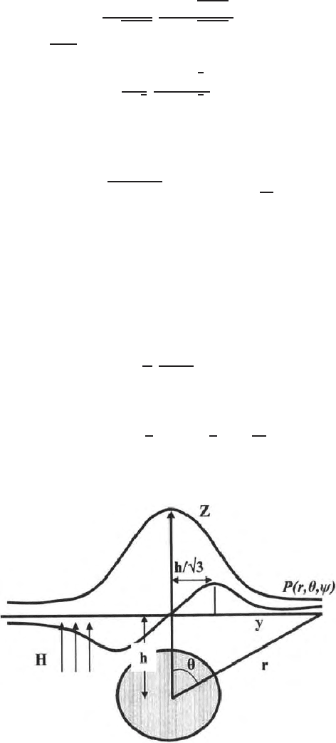
By measuring the vertical component of the anomaly we can pin point
the location of the top of the conductive body. By measuring the horizontal
component and locating the position of
dH
y
H
y
max
from the center of the
body, we can measure the depth of the body since distance of the point of
inflection of the horizontal component from that of the vertical component is
h
√
3
(Fig. 13.15).
13.10.1 Effect of Change in Frequency on the Response Parameter
The value of T is
T=
(n + 1) I
1
(γ
1
a) − γ
1
aI
0
(γ
1
a)
γ
1
aI
0
(γ
1
a) + (n − 1) I
1
(γ
1
a)
. (13.369)
For non magnetic body i.e. for n =
µ
µ
0
=1,
T=
2
γ
1
a
.
I(γ
1
a)
I
0
(γ
1
a)
− 1. (13.370)
Since the frequency chosen is generally small
γ =
iωμ (σ + iω ∈) ≈
iωμσ .
Therefore
13.10 Electromagnetic Induction due to an Infinite Cylinder 433
T=
2
a
√
iωµσ
.
I
1
(a
√
iωµσ)
I
0
(a
√
iωµσ)
− 1. (13.371)
If we write P = a
√
ωμσ as the resp onse parameter,
T=
2
ρ
√
i
.
I
1
P
√
i
I
0
P
√
i
− 1.
=M − iN = A e
−iφ
. (13.372)
Since T is a complex function, it may be written as
|T| =
M
2
+N
2
and φ =tan
−1
N
M
.
Since P, the response parameter, is a combined effect of the radius ‘a’ conduc-
tivity “σ”, frequency “ω ” and magnetic permeability “µ”, the respo nse does
not give any idea about the conductivity of the body at a single frequency.
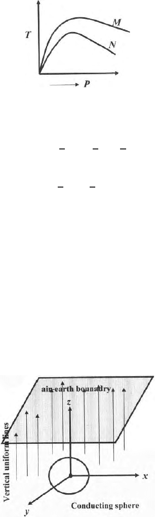
Frequency spectrum for M and N reveals (Fig. 13.16) that sensitivity charac-
teristics M reaches the zone of saturation where as N reaches zero. Therefore,
the operation frequency should b e in the zone where the slope of M and N or
Aandφ are maximum.
Now
T=
2
α
.
I
1
(α)
I
0
(α)
− 1. (13.373)
For small values of α.
I
0
(α)=1+
1
2
α
2
+
1
2
α
4
.
1
2
2
+ (13.374)
and
Fig. 13.15. Variation of horizontal and vertical magnetic field over a buried cylin-
drical inhomogeneity
434 13 Electromagnetic Wave Propagation
Fig. 13.16. Variation of real and imaginary part of T with electromagnetic param-
eter P
I
1
(α)=
1
2
α +
1
2
α
3
1
2
+ (13.375)
Therefore
|T|≈
1
8
α
2
=
1
8
a
2
ωµσ (13.376)
This relation (13.376) holds good unless ω is very large.
13.11 Electromagnetic Response due to a Sphere
in the Field of a Vertically Oscillating Magnetic Dipole
In this problem we shall discuss on the electromagnetic field in the presence
of a spherical body of contrasting electrical conductivity embedded in a host
rock. The source field is assumed to have originated from an oscillating ver-
tical magnetic dip ole. Vector potential approach is adapted here to solve the
boundary value problem. Figure 13.17 shows the geometry of the problem.
Let
Fig. 13.17. A buried conducting sphere in the presence of a vertical uniform mag-
netic field
13.11 Sphere in the Field of a Vertically Oscillating Magnetic Dipole 435
H=curl
A. (13.377)
We can write
H
r
=
1
r
2
sin θ
∂
∂θ
rsinθ
A
ψ
−
∂
∂ψ
r
A
θ
(13.378)
H
θ
=
1
rsinθ
∂
∂ψ
A
r
−
∂
∂r
rsin
A
ψ
(13.379)
and
H
ψ
=
1
r
∂
∂r
r
A
θ
−
∂
∂θ
A
r
. (13.380)
In this problem, the perturbation field will be independent of the azimuthal
angle; therefore
∂
∂ψ
= 0. The vanishing and existing component of the vector
potential and magnetic field are respectively given by
A
r
=0,
A
θ
=0,and
H
r
=0,
H
θ
=0,
H
ψ
=0.Since
A
r
and
A
θ
are both zero, therefore H
ψ
=0.In
this problem
H
r
= H cos θ (13.381)
H
θ
= −
H sin θ (13.382)
H =
k
H
0
(13.383)
where
k is the unit vector along z direction and
r =
ix +
jy +
kz
=
i(rsinθ cos ψ)+
j(rsinθ sin ψ)+
k(rcosθ) . (13.384)
Therefore
dr
dr
=
i(sinθ cos ψ)+
j(sinθ sin ψ)+
k(cosθ) , (13.385)
and
dr
dr
=1. (13.386)
Since
e
r
=
i sin θ cos ψ +
j sin θ sin ψ +
k cos θ, (13.387)
∂r
∂θ
=
i(rcosθ cos ψ)+
j(rcosθ sin ψ)+
k(−rsinθ) , (13.388)
∂r
∂θ
=r,
and
e
θ
=
icosθ cos ψ +
jcosθ sin ψ −
ksinθ. (13.389)
436 13 Electromagnetic Wave Propagation
For the e
ψ
component along the azimuthal angle, we have
∂r
∂ψ
=
i(−rsinθ sin ψ)+
j(rsinθ cos ψ) , (13.390)
∂r
∂ψ
=rsinθ (13.391)
and
e
ψ
= −
isinψ +
jcosψ. (13.392)
We can write down these three equations in the matrix form as
⎡
⎣
sin θ cos ψ sin θ sin ψ cos θ
cos θ cos ψ cos θ sin ψ −sin θ
−sin ψ cos ψ 0
⎤
⎦
⎡
⎣
i
j
k
⎤
⎦
=
⎡
⎣
e
r
e
θ
e
ψ
⎤
⎦
. (13.393)
We can solve for
i,
jand
k using the Cramer’s rule for evaluation of the matrix.
Here the denominator is
D=
⎡
⎣
sin θ cos ψ sin θ sin ψ cos θ
cos θ cos ψ cos θ sin ψ −sin θ
−sin ψ cos ψ 0
⎤
⎦
= 1 (13.394)
and
D
3
=
⎡
⎣
sin θ cos ψ sin θ sin ψe
r
cos θ cos ψ cos θ sin ψe
θ
−sin θ cos ψe
ψ
⎤
⎦
(13.395)
= e
r
cos θ −e
θ
sin θ. (13.396)
Here
k=
|D
3
|
|D|
= e
r
cos θ −e
θ
sin θ (13.397)
and the source vector
H=
k
H
0
=(e
r
cos θ −e
θ
sin θ)H
0
= e
r
(H
rcosθ
)+e
θ
(−H
0
sin θ) . (13.398)
Thus
H
r
=
H
0
cos θ and
H
θ
= −
H
0
sin θ
Let us assume that the source vector has only the ψ component. We can
write
curl
A=
1
r
2
sin θ
∂
∂θ
rsinθ
A
ψ
−
∂
∂ψ
r
A
θ
e
r
+
∂
∂ψ
A
r
−
∂
∂r
rsinθ
A
ψ
r e
θ
+
∂
∂r
r
A
θ
−
∂
∂θ
A
r
rsinθe
ψ
. (13.399)
13.11 Sphere in the Field of a Vertically Oscillating Magnetic Dipole 437
Equation (13.399) can be written as
curl
A=
∂
∂θ
rsinθ
1
2
H
0
rsinθ
e
r
−
∂
∂r
r sin θ
1
2
H
0
r sin θ
r
e
θ
=
1
r
2
sin θ
1
2
r
2
H
0
∂
∂θ
sin
2
θ
e
r
−
1
2
H
0
sin
2
θ
∂
∂r
r
2
e
θ
. (13.400)
⇒curl
A=
1
r
2
sin θ
1
2
r
2
H
0
2sinθ cos θe
r
−
1
2
H
r
0
sin
2
θ
∂
∂r
r
2
e
θ
=H
0
cos θe
r
− H
0
sin θe
θ
. (13.401)
Therefore, the source vector potential
A
ψ
=
1
2
H
0
rsinθe
ψ
.e
iωt
. (13.402)
An uniform alternating primary field can therefore b e obtained from the vector
potential
A.
For this problem, we can write the vector potential
A=
A(r, θ)e
ψ
(13.403)
which changes to
A=−
Asinψ
i+
Acosψ.
j.
If we now operate upon the comp onents in a rectangular coordinate with the
operator ∇
2
and recombine them, it can be shown that Helmholtz equation
changes to the form.
∇
2
A −
A
sin
2
θ
= γ
2
A (13.404)
⇒
1
r
2
∂
∂r
r
2
∂
A
∂r
+
1
r
2
sin θ
∂
∂θ
sin θ
∂
A
∂θ
−
A
sin
2
θ
= γ
2
A. (13.405)
Now substituting
A=r
−1/2
R(r)Θ(θ) (13.406)
and using the method of separation of variable we get
1 −µ
2
∂
2
Θ
∂µ
2
− 2µ
∂Θ
∂µ
+
n(n+1)−
1
1 −µ
2
Θ = 0 (13.407)
438 13 Electromagnetic Wave Propagation
and
d
2
R
dr
2
+
1
r
dR
dr
−
r
2
+
n(n+1)+
1
4
r
2
R=0. (13.408)
The (13.407) is a second order differential equation whose solutions are in
Legendre’s polynomial P
′
n
(cos θ)andQ
′
n
(cos θ). P
′
n
(cos θ) is a better behaved
potential function.
The solution of (13.408) will come in terms o f the modified Bessel’s func-
tion of fractional order in the form
I
n+
1
2
(γr) and K
n+
1
2
(γr) . (13.409)
Therefore, the general solution of the vector potential outside the sphere is
A
0
=
1
2
Hr sin θ +
r
−
1
2
dnI
n+
1
2
(γ
0
r) P
′
n
(cos θ) (13.410)
→ outside the sphere.
A=
r
−
1
2
C
n
I
n+
1
2
(γr) P
′
n
(cos θ) (13.411)
→ inside the sphere.
Since the source potential has sin θ term, the perturbation potential will also
have sin θ term only. Since P
′
1
(cos θ)=sinθ, therefore d
n
= 0, except for
n=1.
Hence
A
0
=
1
2
Hr sin θ +r
−1/2
d
1
I
3/2
(γ
0
r) sin θ (13.412)
and
A = r
−1/2
c
1
I
3/2
(γr)sinθ. (13.413)
Applying the boundary conditions
∂
∂r
(r A
0
)=
∂
∂r
(rA)
µ
0
A
0
= µ
1
A
1
at r = a (13.414)
where ‘a’ is the radius of the sphere.
We get
1
2
Haμ
0
+ μ
0
d
1
a
−1/2
I
3/2
(r
0
a)=μ
1
a
−1/2
c
1
I
3/2
(γa) (13.415)
Ha − d
1
a
−2
= c
1
−
1
2
a
−3/2
I
3/2
(γa)+a
−1/2
γI
′
3/2
(γa)
. (13.416)
From the (13.415) and (13.416), we get
d
1
= −
1
2
Ha
3
)
γaI
′
3/2
(γa) −
2γ −
1
2
I
3/2
(γ
0
a)
γaI
′
3/2
(γa)+
γ +
1
2
I
3/2
(γ
0
a)
*
. (13.417)