Roy K.K. Potential theory in applied geophysics
Подождите немного. Документ загружается.


6.11 Basic Equations in Direct Current Flow Field 149
(i) Radial, perpendi cul ar a nd parallel dipole for 20
◦
≤ θ ≤ 35
◦
(ii) Perpendicular, radial and azimuthal for 35
◦
≤ θ ≤ 65
◦
(iii) Perpendicular, parallel, redial and azimuthal for 65
◦
≤ θ ≤ 75
◦
(iv) Radial and parallel dipoles for 0
◦
≤ θ ≤ 20
◦
(v) Azimuthal and parallel for 75
◦
≤ θ ≤ 90
◦
Bipole-dipole configuration is preferable than that of dipole-dipole for deep
crustal studies. Geometric factors generally used for computation of apparent
resistivities in dipole sounding (6.56 to 6.59) should not be used for small
(00
′
< 4AB) dipole separation. Combination of parallel and perpendicular
dipoles have some logistic advantage in the actual geological ground condi-
tion. Once one knows the orientation of the current dipole, orientation of the
potential dipoles are also known. In a rugged and dense forest region accurate
measurement of dipole angle may be difficult. Measurement of DC dipole field
will r egain its proper pl ace after significant improvements in field logistics as
mentioned and develo pments in interpretation softwares. Fairly detailed expo-
sitions of potential theory related to the direct current flow field are given in
Chaps. 7, 8, 9, 11 and 15.
6.11 Basic Equations in Direct Current Flow Field
1.
j = σ
E (6.60)
2.
→
E
= −gradeφ (6.61)
3.
→
E
=
I
4πσ
.
1
r
3
→
r
(6.62)
4.
→
φ =
I
4πσ
.
1
r
(Point source) (6.63)
5.φ=
→
P
Cosθ
4πσr
2
for DC dipoles.(Dipole source) (6.64)
6.φ= −
Iρ
π
ln r (line source) (6.65)
7.div
→
E
=0or ∇
2
φ = 0 (Laplacian field) (6.66)
8.div∇
2
φ = ρ (Poissonian field) (6.67)
9.Curl
→
E
= 0 (6.68)
10.divj= −
∂q
∂t
(6.69)
11.J
n
1
= J
n
2
(6.70)
12.ρ
1
tan θ
1
= ρ
2
tan θ
2
(6.71)
150 6 Direct Current Flow Field
6.12 Units
σ → mho/meter(Siemen)
ρ → Ohm–meter
R → Ohm
J → Amp/me ter
2
φ → V olt/Milliv olt
E → V olt/meter

7
Solution of Laplace Equation
In this chapter solutions of Laplace equation in cartisian, cylindrical p olar
and spherical polar coordinates using the method of separation of variables
are discussed in considerable details. The nature of solution of boundary value
problems in potential theory is introduced. The nature of Bessel’s function ,
modified Bessel’s function, Legendre’s Polynomial and Associated Legendre’s
Polynomial are shown. A brief discussion on Spherical Ha rmonics is given.
7.1 Equations of P oisson and Laplace
The electric displacement vector is
D=∈
E { (4.4.)} where
D is the electric
displacement,
E is the electric field and ∈ is the electrical permittivity of
a medium. In addition to the constitutive relation, we use the Gauss’s flux
theorem of total normal induction on a closed surface due to a charge inside
the enclosed volume and it is given by
s
D
n
.ds =
div
D.dv = q =
ρdv (7.1)
where ρ is the volume density of charge and dv is the infinitesimal volume.
Hence
∇.D=ρ (7.2)
⇒∇.(∈ E) = ρ
⇒∇.(−∈∇φ)=ρ
⇒−∈div grad φ = ρ
⇒∇
2
φ = −
ρ
∈
(7.3)
=0whenρ =0.
152 7 Solution of Laplace Equation
In a source free region (Fig. 6.2 a and b)
−∈∇
2
φ =0. (7.4)
For a nonhomogenous but isotropic dielectric (7.4) becomes
∂
∂x
∈
∂φ
∂x
+
∂
∂Ψ
∈
∂φ
∂y
+
∂
∂x
∈
∂φ
∂x
=0. (7.5)
For a homogenous and isotropic dieletric
∂
2
φ
∂x
2
+
∂
2
φ
∂y
2
+
∂
2
φ
∂z
2
=0. (7.6)
For three principal axes anisotropy (7.5) will be
∂
∂x
∈
xx
∂φ
∂x
+
∂
∂y
∈
yy
∂φ
∂y
+
∂
∂z
∈
zz
∂φ
∂x
=0. (7.7)
7.2 Laplace Equation in Direct Current Flow Domain
When current is flowing out of a closed region, the flow of charge will be
guided by the relation
div
J=−
∂ρ
∂t
(7.8)
where ρ is the volume density of charge in Coulomb/meter
3
and
J is current
density in ampere/meter
2
. Since this rel ation satisfies the law of conserva-
tion of charge, it is termed as the equation of continuity. In a source free
region
div
J = 0 (7.9)
where
J = σ
E = −σg radφ,whereφ is the potential (in volt) and
Eisthe
electric field in volt/meter. Equation (7.9) can be written as
div (σ grad φ) = 0 (7.10)
⇒ grad (σ)gradφ +(σ)div grad φ =0. (7.11)
For an homogeneous and isotropic medium (7.11) reduces to Laplace equation
∇
2
φ =0. (7.12)
Non Laplacian character of (7.11) is demonstrated in Chap. 8.
7.3 Laplace Equation in Generalised Curvilinear Coordinates 153
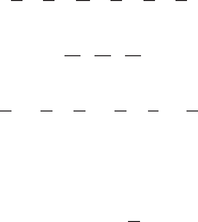
Fig. 7.1. A cuboid with curve sides to represent the curvilinear coordinates
7.3 Laplace Equation in Generalised Curvilinear
Coordinates
Laplace equations in cartesian, cylindrical polar and spherical polar coordi-
nates can be expressed from the expression of Laplace equation in generalized
curvilinear coordinates (Fig. 7.1).
In orthogonal curvilinear co o rdinate, the Laplace equation is
∇
2
φ =
1
h
1
h
2
h
3
∂
∂u
1
h
2
h
3
h
1
∂φ
∂u
1
+
∂
∂u
2
h
1
h
3
h
2
∂φ
∂u
2
+
∂
∂u
3
h
1
h
2
h
3
.
∂φ
∂u
3
. (7.13)
Here the value of h
1
,h
2
,h
3
and u
1
,u
2
and u
3
can be expressed as :
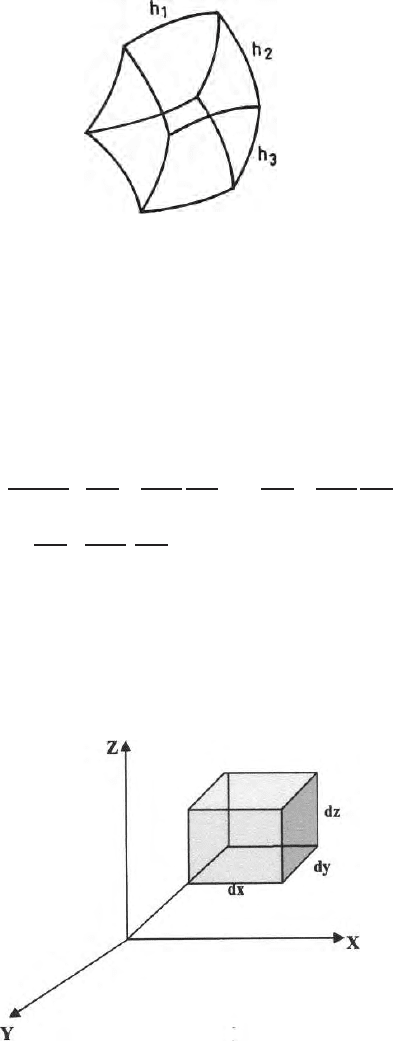
(a) In cartesian coordinates (Fig. 7.2)
u
1
=x, u
2
=y and u
3
=z
h
1
=1, h
2
=1, and h
3
= 1 (7.14)
Fig. 7.2. A three dimensional elementary volume in Cartisian co ordinatea (x,y,z)
154 7 Solution of Laplace Equation
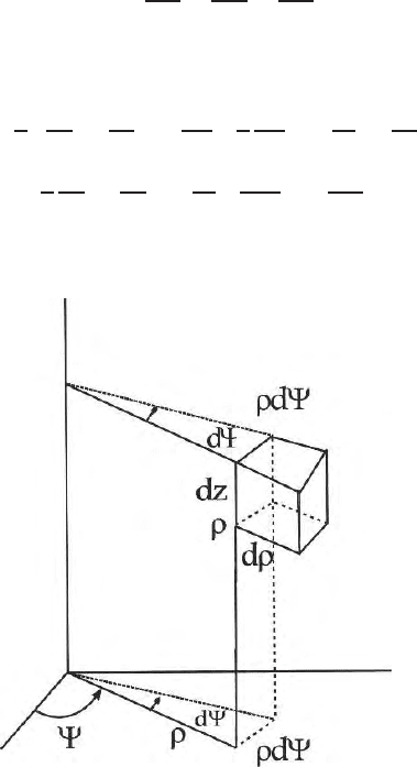
(b) in cylindrical polar coordinates (Fig. 7.3)
u
1
= ρ, u
2
=Ψ and u
3
=z
h
1
=1, h
2
= ρ and h
3
= 1 (7.15)
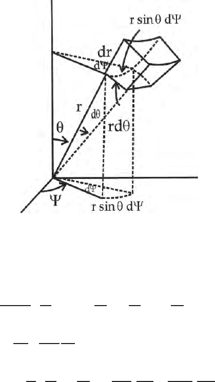
(c) In spherical p olar coordinates (Fig. 7.4)
u
1
=r, u
2
= θ and u
3
= ψ
h
1
=1, h
2
=r, and h
3
=rsinψ. (7.16)
Therefore, the expressions for the Laplace equation in three coordinate sys-
tems are respectively given by
(a)
∇
2
φ =
∂
2
φ
∂x
2
+
∂
2
φ
∂y
2
+
∂
2
φ
∂z
2
= 0 (7.17)
in Cartesian co ordinate, where φ =f(x, y, z).
(b)
∇
2
φ =
1
ρ
∂
∂ρ
ρ
∂φ
∂ρ
+
∂
∂Ψ
1
ρ
∂φ
∂Ψ
+
∂
∂z
ρ
∂φ
∂z
=0
⇒
1
ρ
∂
∂ρ
ρ
∂φ
∂ρ
+
1
ρ
2
∂
2
φ
∂Ψ
2
+
∂
2
φ
∂z
2
= 0 (7.18)
in cylindrical polar coordinates where φ =f(ρ, ψ, z.).
Fig. 7.3. A three dimensional elementary volume in cylindrical polar coordinates
(r, ψ,z)
7.3 Laplace Equation in Generalised Curvilinear Coordinates 155
Fig. 7.4. A three dimensional elementary volume in spherical polar coordinates
(r, θ, ψ)
(c)
∇
2
φ =
1
r
2
sin θ
∂
∂r
r
2
sin θ
∂φ
∂r
+
∂
∂θ
sin θ
∂φ
∂θ
+
∂
∂Ψ
1
sin θ
∂φ
∂ψ
=0
⇒
1
r
2
∂
∂r
r
2
∂φ
∂r
+
1
sin θ
.
∂
2
φ
∂θ
2
+
1
sin
2
θ
.
∂
2
φ
∂ψ
2
= 0 (7.19)
in spherical po lar co ordinates where φ =f(r, θ, ψ). Most of the geophysical
problems, dealing with scalar potential field satisfy Laplace equation in a
source free region i.e. the region which excludes the source (field exists but
not the source) (Fig. 2.5 a and 6.2 a,b). Therefore, the solution of Laplace
equation forms a significant part of the potential theory in geophysics. In this
chapter we shall deal with the solution of Laplace equation by the method of
separation of variable in (i) cartesian (ii) cylindrical polar and (iii) spherical
polar coordinates depending upon the nature of the problems. One has to
choose the proper coordinate system for solving a particular problem A few
simpler pro b lems are included.
156 7 Solution of Laplace Equation
7.4 Laplace Equation in Cartesian Coordinates
The solution of the Laplace equation by the method of separation of variables
in cartesian coordinate is demonstrated in this section.When potential φ is a
function of x, y and z where X, Y, Z are independent variables, we can write:
φ = X (x) Y (y) Z (z) (7.20)
and
∂φ
∂x
=YZ
∂X
∂x
(7.21)
or,
∂
2
φ
∂x
2
=YZ
∂
2
X
∂x
2
. (7.22)
Substituting these values in (7.17) we get
∇
2
φ =
∂
2
φ
∂x
2
+
∂
2
φ
∂y
2
+
∂
2
φ
∂z
2
= 0 (7.23)
YZ
d
2
X
dx
2
+ ZX
d
2
Y
dy
2
+ XY
d
2
Z
dz
2
=0. (7.24)
Dividing the whole (7.24) by XYZ, we get:
1
X
.
d
2
X
dx
2
+
1
Y
.
d
2
Y
dy
2
+
1
Z
.
d
2
Z
dz
2
=0. (7.25)
The sum of these terms will never be zero unless each individual terms are
constants and the sum of these constants is zero i.e., if
1
X
.
d
2
X
dx
2
= α
2
1
Y
.
d
2
Y
dy
2
= β
2
1
Z
.
d
2
Z
dz
2
= γ
2
(7.26)
then
α
2
+ β
2
+ γ
2
=0. (7.27)
We shall now examine the nature of the expressions for potentials for their
depen d ence on the different axes:
7.4.1 When Potential is a Function of Vertical Axis z, i.e., φ =f(z)
The Laplace equation reduces d own to
∂
2
φ
∂z
2
= 0 and the solution is
φ = cz + d (7.28)
7.4 Laplace Equation in Cartesian Coordinates 157
where c and d are two arbitrary constants. Here potential is increasing with z,
i.e., higher the value of z, higher will be the potential. One encounters this kind
of situation while computing gravitational potentials due to a hypothetical
infinite plate. Here
E=−
∂φ
∂Z
= c (7.29)
i.e., the field is constant at any distance from the plane.
7.4.2 When Potential is a Function of Both x and y, i.e., φ =f(x, y)
Putting φ = X (x) Y (y)
The Laplace equation reduces down to:
1
X
.
d
2
X
dx
2
+
1
Y
.
d
2
Y
dy
2
=0. (7.30)
If
1
X
.
d
2
X
dx
2
= α
2
, then
1
Y
.
d
2
Y
dy
2
= −α
2
. (7.31)
And if
1
X
.
d
2
X
dx
2
= −β
2
, then
1
Y
.
d
2
Y
dy
2
= β
2
. (7.32)
Therefore, we can write:
d
2
X
dx
2
− α
2
X=0
d
2
Y
dy
2
+ α
2
Y = 0 (7.33)
The solutions are:
X=e
αx
, e
−αx
, cosh αx, sinh αx (7.34)
and
Y=e
iαy
, e
−iαy
, cos αy, sin αy
The most general solution of Laplace equation for these two equations are:
φ =
∞
n=0
a
n
e
α
n
x
+b
n
e
−α
n
x
(c
n
cos α
n
y+d
n
sin α
n
y) (7.35)
and
φ =
∞
n=o
(a
n
cos β
n
y+b
n
sin β
n
y) (c
n
cosh α
n
x+d
n
sinh α
n
x) (7.36)
158 7 Solution of Laplace Equation
7.4.3 Solution of Boundary Value Problems in Cartisian
Coordinates by the Method of Separation of Variables
Let us find out the potential at any point in a two dimensional space when
the size of the conductor and the potentials on the boundaries are prescribed.
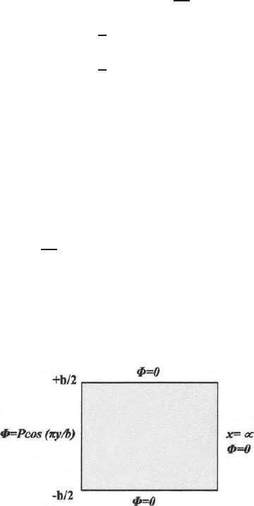
Problem 1
A rectangular block of a conductor of thickness ‘b’ is placed in the xy plane.
The prescribed values at different bou ndaries are:
x=∞, φ =0
x=0, φ =Pcos
πy
b
′
y=−
b
2
, φ =0
y=+
b
2
, φ =0
Find the potential at any point in the r ectangular plate.
Figure (7.5) shows the nature of the problem. Since φ =0atx=∞,the
general solution of the two dimensional potential problem takes the form:
φ =
∞
n=0
b
n
e
−α
n
x
(c
n
cosh α
n
y+d
n
cinα
n
y) . (7.37)
Applying the second boundary condition, we get :
Pcos
πy
b
=
(c
′
n
cos α
n
y+d
′
n
sin α
n
y) (7.38)
where c
′
n
=b
n
c
n
and d
′
n
=b
n
c
n
. These are arbitrary constants to b e deter-
mined from the boundary conditions. Since the source potential contains ‘cos’
term,wehavetodropthe‘sin’termsfromthe solution. Therefore, th e expres-
sion for the potential reduces to:
Fig. 7.5. A t wo dimensional Dirichlet’s problem with potentials prescribed in all
the boundaries