Roy K.K. Potential theory in applied geophysics

Подождите немного. Документ загружается.

6.8 Current Flow Inside the Earth 139

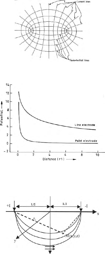
Equation (6.35) generates elliptic equipotential lines (Fig. 6.11). Therefore

current lines will be hyperbolic.

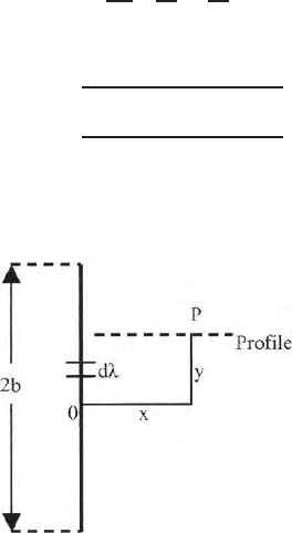
Integral transform of Roy and Jain (1961) can be stated as follows. Let a

point electrode in the vicinity of a two dimensional structure striking in the

y direction, produce a potential φ (x, y ) along a proﬁle in the y-direction. The

proﬁle goes through a point P at a distance x from the electrode. Then the

transform

φ (x) =

∞



−∞

φ (x, y) dy (6.36)

generates the potential, that would be prod uced at P by a line electrode

parallel to the proﬁle but placed in the p osition o f point electrodes. The

total current in the point electrode is the curren t per unit length of the line

electrode. Figure 6.12 shows the variation of potential with distance due to a

point and a line electrode.

6.8 Current Flow Inside the Earth

Potential at a point M (Fig. 6.13) in a semi inﬁnite medium of resistivity ρ

due to a source +I and sink (−I) on the surface of the earth is given by

2π



−



(6.37)

where



(L/2+x)

+ y

+ z

(6.38)



(L/2 − x)

+ y

+ z

(6.39)

where L is the electrode separation. Here.

Fig. 6.10. A ﬁnite line electrode of length 2b carrying current I

140 6 Direct Current Flow Field

Fig. 6.11. Current lines and equipotential lines due to a line current source of ﬁnite

length

Fig. 6.12. Shows the v ariation of potential with distance from a point and a line

electrode

Fig. 6.13. Shows the nature of direct current ﬂow through a homogeneous medium

6.8 Current Flow Inside the Earth 141



= −

∂φ

∂x



= −

∂φ

∂y

(6.40)



= −

∂φ

∂z

are the current densities along the x, y and z directions when current is ﬂowing

through a homogenous medium. Here



2π

)

+ x

−

− x

(6.41)



2π



−

(6.42)



2π



−

(6.43)



J =



+ J

. (6.44)

If we bring the point M on the YZ plane then x = 0 and r

reduces

to the form.

2π

(L/2)

+ y

+ z

. (6.45)

Current density on the surface on the earth at z = 0 is given by

(6.46)

and at a depth h is

2π







+ h

. (6.47)

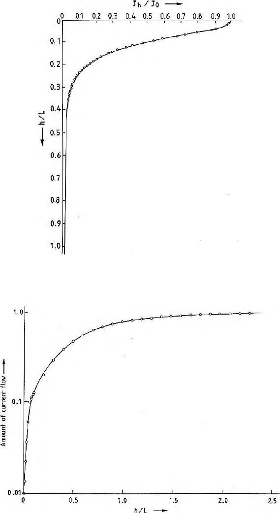
The ratio of the current density at a certain depth h and that on the surface

is given by



1+(2h/L)



3/2

. (6.48)

Figure 6.14 shows the variation of current density with depth in

plot.

Flow of current upto the depth h is given by

142 6 Direct Current Flow Field

Fig. 6.14. Shows the variation of current density with depth in a xz plane passing

through y = 0 at the centre of the electrode conﬁguration

Fig. 6.15. Amount of current ﬂows through the earthwithdepthandtherelation

with electrode separation

6.9 Refraction of Current Lines 143

2π



y=−α



z=0

dydz







+ y

+ z



3/2

(6.49)







+ z

tan

−1

(6.50)

tan

−1

. (6.51)

This gives the total amount of current ﬂowing between the surface at any

particular depth. Figure 6.15 shows the variation of

with h/L. It is observed

that most of the current is concentrated near the surface.

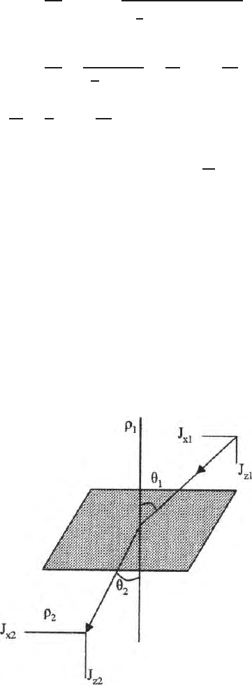
6.9 Refraction of Current Lines

Direct currents get refracted across a contact of two media of diﬀerent r esis-

tivities and follow ‘tan’ law unlike ‘sine’ law for seismic or elastic waves. Two

homogeneous and isotropic media of resistivity ρ

and ρ

are having a hori-

zontal contact Fig. 6.16 of inﬁnite horizontal extent.

Current with a current density J

is incident on the horizontal surface at an

angle θ

. J

and J

are respectively the horizontal and vertical components.

This current element is at an angle θ

with the vertical.

Fig. 6.16. Shows the refraction of the current lines at the boundary between the

two media having resistivity ρ

and ρ

144 6 Direct Current Flow Field

Now for direct current ﬂow ﬁeld, the potential must be continuous across

the boundary i.e., ϕ

= ϕ

and the normal component of the current densities

and J

must be continuous ac ross the boundary.

In terms of electric ﬁeld, we can write,

= E

and σ

= σ

. (6.52)

From (6.52), we can write

= J

and J

= J

. (6.53)

From the two equations, we get

)=ρ

) ⇒ ρ

tan θ

= ρ

tan θ

. (6.54)

6.10 Dipole Field

Figure 6.7 shows the nature of the direct current ﬂow ﬁeld for DC dipoles

when the distance between the two current electrodes are signiﬁcantly less

in comparison to the distance where we measure the ﬁeld. The essential dif-

ferences between a dipole and a bipole ﬁeld are (i) dipole ﬁelds die down at

a much faster pace. DC dipole potential varies as

with distance and ﬁeld

varies as

with distance. Expression for dipole ﬁelds and potential are pre-

sented in Chap. 4. Expressions for potentials in dipoles in electrostatic ﬁeld

and direct current ﬂow ﬁelds are a nalogous. (Chap. 4, (4.30) and (4.31)). Only

q the charge strength is replaced by current strengths I and ∈, the electrical

permittivity is replaced by electrical conductivity σ.

D.C. dipole ﬁelds are being used by the geophysicists primarily to have

informarion of the subsurface from a relatively greater depth. Deeper probing

is possible by sending more current through the earth and measuring poten-

tials far away from the current dipo le.

Direct current d i pole-dipole conﬁgurations for measuring the electrical

resistivity of the earth’s crust is known from the works o f Alpin et al (1950),

Jackson (1966), Keller et al (1966), Anderson and Keller (1966), Zohdy (1969),

Alfano (1980).

Important D.C. dipole conﬁgurations for deeper probing (sounding) are,

(I) equatiorial (ii) azimuthal (iii) parallel (iv) perpendicular and (v) axial.

dipoles (Fig. 6.17 a, b, c, d, and e). Important D.C dipole conﬁguration for

studying the lateral heterogeneites is the collinear dipole dipole conﬁguration

(Fig. 6.18). Figure 6.18 also shows the data plotting points in the pseudosec-

tion form.

In bipole-dipole conﬁguration, the length of the current dipole AB may be

much larger than the potential dipole MN (Fig. 6.17).

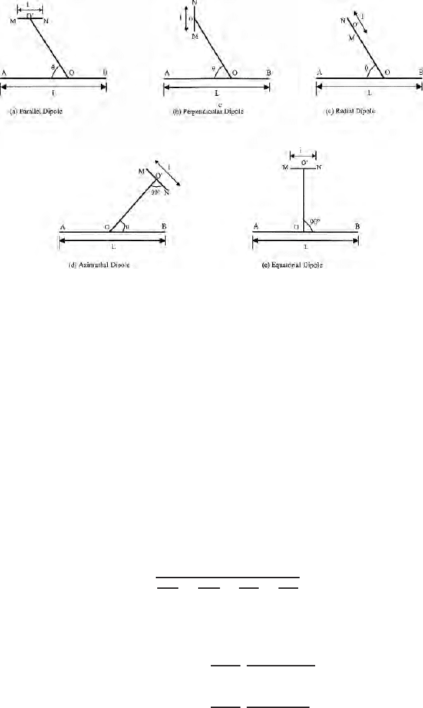
6.10 Dipole Field 145

Fig. 6.17. Show the DC dipole conﬁguration; (a) Parallel dipole conﬁguration where

current dipole and potential dipole are parallel; the line joing the midpoints of

the current and potential electrode is making an angle θ not equal to 90

◦

;(b)

Perpendicular dipole conﬁguration; here p otential dipole is at right angles to the

current dipoles at all dipole angles; (c) Radial dipole conﬁguration: Here potential

dipole is in the same line which joins the midpoints of the current and potential

electrodes at all dipole angles; (d) Azimuthal dip ole conﬁguration; here p otential

dipole is at right angles to the line joining the mid points of the current and potential

dipoles; (e) Equatorial dipoles; here the current and potential dipoles are parallel

and the dipole angle is 90

◦

For dipole dipole system AB should be nearly equal to MN. Equato-

rial dipole and azimuthal dipoles are used quite frequently in dipole survey

because these data can directly be converted to Schlumberger data and can be

interpreted.

The general expression for the geometric factor for all the electrode con-

ﬁgurations is

K =

2π

−

(6.55)

The approximate geometric factors for diﬀeren t bipole-dipole conﬁgurations

are

parallel

2πr

3cos

θ − 1

(6.56)

perpendicular

2πr

sin θ cos θ

(6.57)

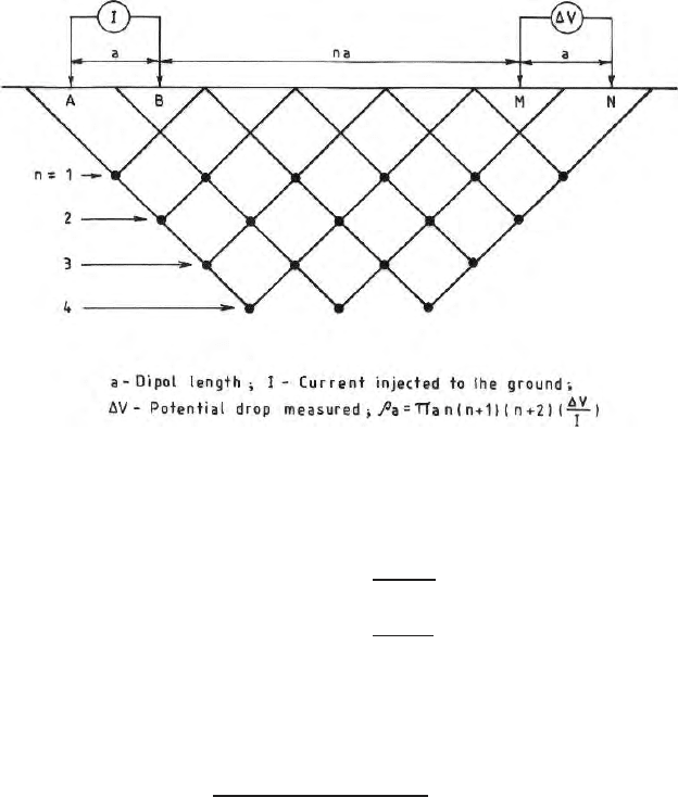
146 6 Direct Current Flow Field

Fig. 6.18. Sho ws the collinear dipole dipole conﬁguration; here current and poten-

tial electrode pairs are in the same line; electrode separations are increased with

higher values of n; pseudo net is for plotting data

radial

πr

L cos θ

. (6.58)

azimuthall

2πr

L sin θ

. (6.59)

(Aplin 1950, Bhattacharyya and Patra, 1968 and Koefoed, 1979)

Here θ is the dipole angle. L and r a re respectively the current dipole

length and the dipole separation. The percentage discrepancy

δ =

actual

− K

approximate

actual

× 100%

between the actual and approximate geometric factors (6.55 to 6.59) can be

very high in some ca ses. This discrepancy is signiﬁcant for bip ole-dipole sys-

tem. For dipole -dipole system, when AB

∼

MN, this discrepancy δ goes down

signiﬁcantly. Figure 6.19 shows the decrease in the percentage discrepancy δ

computed for an homogenous earth model as well as for parallel dipole con-

ﬁguration for MN = 300 meters, ρ = 1000 ohm – meters for diﬀerent current

dipole lengths and dipole separations and current sent through the ground

was assumed to be one ampere.

Discrepancy between the actual and approximate geometric factor reduces

down signiﬁcantly with increasing dipole separation OO’ where O and O

′

are

the mid points of the current and potential dipoles.

DC dipole ﬁeld measurement is essentially an attempt to measure a man

made ﬁeld obtained by a generator driven power at a far of point. Diﬃcult

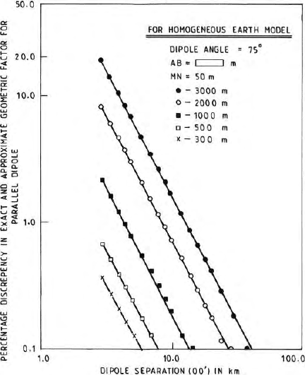
6.10 Dipole Field 147

Fig. 6.19. Sho ws the discrepancy between the exact and approximate geometric

factor in the case of parallel dipole for diﬀerent current dipole lengths and dipole

separations (OO’); This ﬁgure is for homogenuous and isotropic half space and dipole

angle 75

◦

ﬁeld logistics to layout several kilometers of ﬁeld cables for deep er probing in

case Schlumberger or Wenner array could be avoided by separating the current

and potential dipoles as two independent units. Advent of sophisticated and

accurate global positioning system (GPS), distance communication system

and mobile telephones signiﬁcantly reduced the ground hazards in measuring

dipole ﬁelds and subsequent data analysis specially for earth’s crustal.studies.

Cultural noise problem is signiﬁcantly low in this case in comparison to

what one expects for audiofrequency magnetotelluric survey.

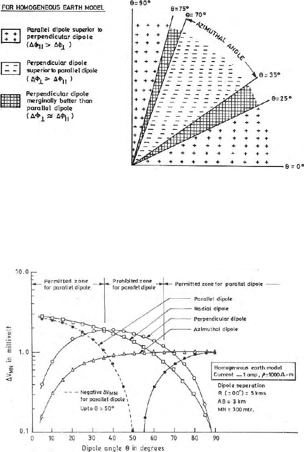
Parallel dipole conﬁguration does not work at dipole angle nearly 55

◦

(Keller 1966, θ =53

◦

′

, Zohdy 1969, θ =54

◦

′

, Alpin et al 1950,

θ =54

◦

′

′′

, Das and Verma, 1980 θ =54

◦

–55

◦

). At this angle E

,the

parallel curr ent dipole component of the electric ﬁeld is zero. Therefore, any

measurement in the vicinity of this dipole angle is unreliable. It is now realised

that not only one should avoid θ =53

◦

, there is a big zone from θ =35

◦

θ =65

◦

, where parallel dipole does not work. It is termed as the prohibitive

zone (Fig. 6.20) for parallel dipole. Permitted zones for parallel dipole system

are θ =0

◦

to 35

◦

and 65

◦

to 90

◦

. Therefore, the recommended prescription

for use of bip ole-dipole conﬁgurations for various dipole angle are (Fig. 6.21):

148 6 Direct Current Flow Field

Fig. 6.20. Shows the diﬀerent working zones for parallel and perpendicular dipoles;

Parall el dipole works for dipole angle 0

◦

to 35

◦

and 70

◦

to 90

◦

and perpendicular

dipole works best within the dipole angle 35

◦

to 70

◦

Fig. 6.21. Shows the v ariations of potentials for diﬀerent dipole angles and diﬀerent

dipole conﬁgurations in a homogeneous and isotropic half space; it is an approxi-

mate guideline for choice of DC dipoles for diﬀerent dipole angles, computation of

potentials is made for current dipole length = 3 km, potential dipole length = 300

meter and dipole separation R = OO

′

=5km