Roff D.A. Modeling Evolution: An Introduction to Numerical Methods
Подождите немного. Документ загружается.

> print(Best.E)# Print optimum E
[1] 0.5651338
The results indicate that under this scenario a medium reproductive effort is
optimal. Benton and Grant (1999) explored a range of scenarios in which both
the density-dependent function and traits affected were varied. The results are
given in Table 1 of their paper: I suggest that the reader modify the above coding
to replicate the results of that table.
3.7 Scenario 5: A two stage model
The primary purpose of this scenario is to illustrate the importance of correctly
setting the number of generations over which the invader population growth rate
is estimated. The problem is to estimate the optimal proportion of a population
delaying maturity (or equivalently the proportion of immatures entering diapause
or dormancy as found in many invertebrates and plants). For a detailed discussion
of the model see van Dooren and Metz (1998). In this case I present the elasticity
analysis first. Because the coding for multiple invasibility analysis is essentially the
same as in previous scenarios, I have omitted it here.
3.7.1 General assumptions
1. The population consists of two stages with reproduction in the second stage.
2. A proportion of the first stage remains in that stage for more than one popula-
tion cycle.
3. Fecundity is density dependent.
3.7.2 Mathematical assumptions
1. The proportion showing delayed maturity is P and the survival between stages
is S.
2. Fecundity is determined by the Ricker function as ae
bA
t
.
The matrix model is thus
I
tþ1
A
tþ1
¼
SP ae
bA
t
Sð1 PÞ 0
I
t
A
2
ð3:33Þ
Parameter values are set at S ¼ 0.8, ¼ 18, and b ¼ 0.01. The dynamics of the adult
population depend critically on the proportion delaying maturity. Low values of P
produce cyclical behavior and larger values produce a stable equilibrium, with the
time attaining the equilibrium becoming shorter as P gets bigger (Figure 3.13). As a
consequence the dynamics of the resident and invader populations, both may
208 MODELING EVOLUTION

Generation
Generation
GenerationGeneration
0
0
0 50 100 200
100 200
Adults
Adults
0 50 100 200
Adults
0 50 100 150
Adults
300 400 500
20 40 60 80 100 0 20 40 60 80 100
0 20406080100
0 20406080100
Figure 3.13 Population dynamics for the stage‐dependent model of Scenario 5. Values of
P
from right to left and top to bottom are 0.1, 0.5, 0.7, and 0.9.
rm(list=ls()) # Clear workspace
par(mfrow=c(2,2)) # Divide graphics page into quarters
ALPHA <- 18 ; BETA <- 0.01; S <- 0.8 # Parameter values
Ps <- c(.1,.5,.7,.9) # Values of P
for ( Ith.P in 1:4) # Iterate over P values
{
P <- Ps[Ith.P] # Select P value
Stage <- c(0,1) # Start with one Adult
# Initialize matrix
Stage.matrix <- matrix(c(S*P, S*(1-P), ALPHA*exp(-BETA*Stage
[2]),0),2,2)
Maxgen <- 100 # Nos of generations to run simulation
Store.Stage<- matrix(0,Maxgen,2) # Preallocate space for storage
Store.Stage[1,] <- Stage # Store generation 1
for (Igen in 2:Maxgen) # Iterate over generations
{
Stage <- Stage.matrix%*%Stage # New matrix
Stage.matrix[1,2] <- ALPHA*exp(-BETA*Stage[2]) # Apply DD func-
tion
Store.Stage[Igen,]<- Stage # Store data
} # End of Igen loop
plot(seq(from=1, to=Maxgen), Store.Stage[,2],xlab=’Genera-
tion’, ylab=’Adults’, type=’l’)
} # End of Ith.P loop
fluctuate, leading to uncertainty in the outcome of an invasion unless the time
span is sufficiently long. Further, the variable dynamics may generate polymorph-
isms or multiple equilibria.
3.7.3 Elasticity analysis
Program coding follows the same pattern as in the previous scenario, except that
the density dependence function is placed directly in the function POP.DYNAM-
ICS. The line of coding shown in bold font is critical in this case.
R CODE:
rm(list¼ls()) # Clear workspace
par(mfrow¼c(1,1)) # Divide graphics page into quarters
POP.DYNAMICS <- function(P, P.invader.coeff)
{
P.resident <- P # Resident delay
P.invader <- P*P.invader.coeff # Invader delay
ALPHA <- 18; BETA <- 0.01; S <- 0.8 # parameter values
Resident.Stage <- c(1,1) # Initial resident population
Invader.Stage <- c(1,1) # Initial invader population
# Initiate resident and invader matrices
Resident.matrix <- matrix(c(S*P.resident, S*(1-P.resident),
ALPHA*exp(-BETA*Resident.Stage[2]),0),2,2)
Invader.matrix <- matrix(c(S*P.invader, S*(1-P.invader),
ALPHA*exp(-BETA*Invader.Stage[2]),0),2,2)
Maxgen <- 100 # Generations with resident alone
Store.Invader <- matrix(0,Maxgen,2)
Store.Invader[1,] <- Invader.Stage
for (Igen in 2:Maxgen) # Iterate until resident is stable
{
Resident.Stage <- Resident.matrix%*%Resident.Stage # New matrix
Resident.matrix[1,2] <- ALPHA*exp(-BETA*Resident.Stage[2])
# DD effect
} # End of 1
st
Igen loop
# Now enter invader
Pop.invader <- matrix(0,Maxgen,1)
Maxgen <- 100 # Set number of generations for invasion
for (Igen in 1:Maxgen) # Iterate over generations after invasion
{
N <- Resident.Stage[2]þ Invader.Stage[2]# Adult population size
Resident.matrix[1,2] <- ALPHA*exp(-BETA*N) # Apply DD to resident
Invader.matrix[1,2] <- ALPHA*exp(-BETA*N) # Apply DD to invader
# New matrices
Resident.Stage <- Resident.matrix%*%Resident.Stage
Invader.Stage <- Invader.matrix%*%Invader.Stage
210 MODELING EVOLUTION
Pop.invader[Igen] <- Invader.Stage[2] # Store invader adult pop
} # End of 2nd Igen loop
Generation <- seq(from¼20, to¼Maxgen) # Generation vector
# Get invasion exponent from linear regression
Invasion.model <- lm(log(Pop.invader[20:Maxgen])Generation
[20:Maxgen])
Elasticity <- Invasion.model$coeff[2]
} # End of POP.DYNAMICS
#################### MAIN PROGRAM ####################
par(mfrow¼c(2,2)) # Divide graphics page into 4 quadrats
# Call uniroot to find optimum
Optimum <- uniroot(POP.DYNAMICS, interval¼c(0.1,0.6),0.995)
Best.P <- Optimum$root # Store optimum P
print(Best.P) # Print out optimum
N.int <- 30 # Nos of intervals for plot
P <- matrix(seq(from¼0.1, to¼.6, length¼N.int), N.int,1)
Elasticity <- apply(P,1,POP.DYNAMICS, 0.995)
plot(P, Elasticity, type¼’l’)
lines(c(.01,.9), c(0,0)) # Add horizontal line at zero
# Now plot Invasion exponent when resident is optimal
Coeff <- P/Best.P # Convert P to coefficient
Invasion.coeff <- matrix(0,N.int,1)
for (i in 1:N.int){ Invasion.coeff[i] <- POP.DYNAMICS(Best.P,
Coeff[i])}
plot(P, Invasion.coeff, type¼’l’)
points(Best.P,0, cex¼2)
OUTPUT:
> print(Best.P) # Print out optimum
[1] 0.3506968
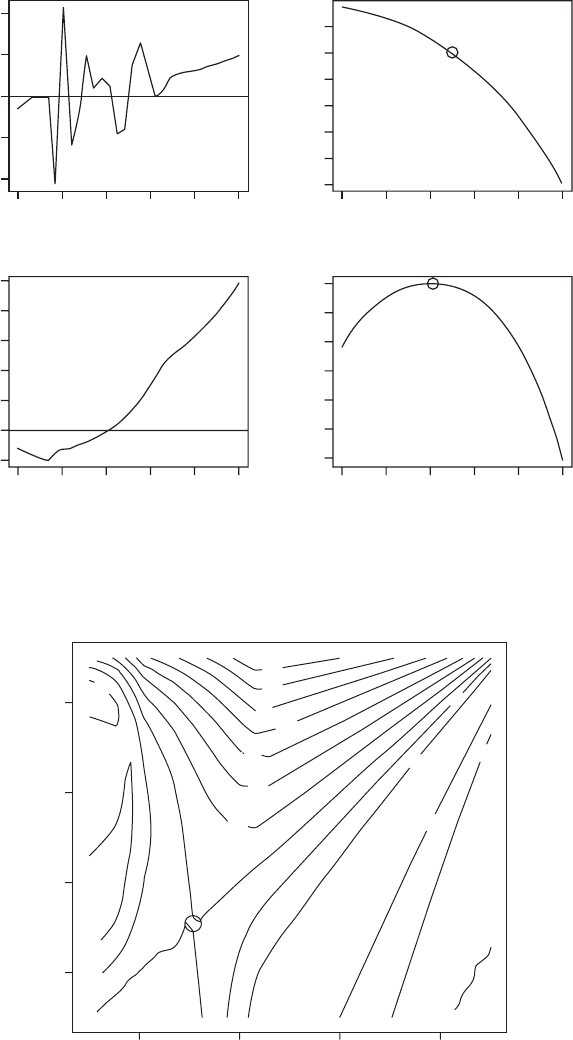
The R function uniroot is successful in finding a root but it is quite clear from the
graphical output (upper panels of Figure 3.14) that this is not the optimum. At first
glance one might suppose that there are multiple ESS values, however, this
variation disappears if the invader population is monitored for 2,000 generations
and a single ESS value of 0.307579 is found (lower panels of Figure 3.14).
3.7.4 Pairwise invasibility analysis
Coding is omitted as it is essentially the same as in the previous two scenarios.
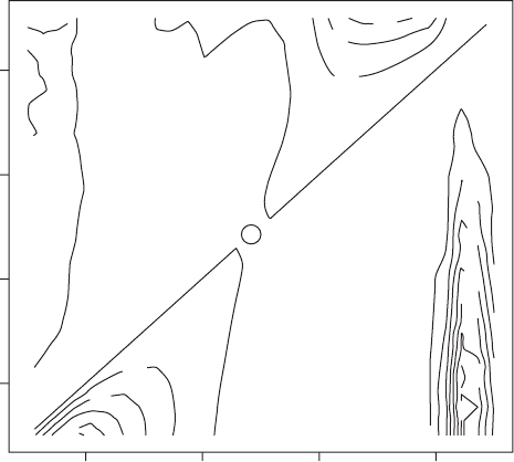
What is important is that the plot generated after only 100 generations gives a
remarkably accurate graphical estimate (Figure 3.15), as indicated by the super-
imposed plot from the elasticity analysis.
INVASIBILITY ANALYSIS 211

P
0.1 0.2 0.3 0.4 0.5 0.6
P
0.1 0.2 0.3 0.4 0.5 0.6
P
0.1
–0.012
–2e-04 2e-04
Elasticity
Elasticity
6e-04 1e-03
–0.002 0.000 0.002
–0.008
Invasion.coeff
Invasion.coeff
–0.004 0.000 –0.025 –0.015 –0.005 0.005
0.2 0.3 0.4 0.5 0.6
P
0.1 0.2 0.3 0.4 0.5 0.6
Figure 3.14 Elasticity analysis of Scenario 4. Top row shows results when invader is
monitored for 100 generations and bottom row shows the results of monitoring for 2,000
generations.
Resident
0.2
0.2 0.4
Invader
0.6 0.8
0.4 0.6 0.8
–0.14
–0.12
–0.1
–0.08
–0.06
–0.04
0.04
0.04
0.02
0.02
–0.02
0.02
0.04
0.04
0
0
–0
Figure 3.15 Pairwise invasibility plot of Scenario 5. The invading population was monitored
for only 100 generations. Superimposed is the value (circle) predicted from the elasticity
analysis run for 2,000 generations.
212 MODELING EVOLUTION

3.8 Scenario 6: A case in which the putative ESS is not stable
This scenario is discussed in detail in White et al. (2006). The present model is
slightly modified to ensure that population size is reasonably large (>20). The
results illustrate the importance of both an invasibility analysis and an elasticity
analysis. The coding is essentially same as in previous scenarios.
3.8.1 General assumptions
1. Population size is governed by both density dependent and density-indepen-
dent factors.
2. The density-independent components of fecundity and survival are negatively
related.
3. The above function generates complex population dynamics.
3.8.2 Mathematical assumptions
1. Population size at time t þ 1, N
tþ1
, is given by the equation
N
tþ1
¼ N
t
ðae
bN
t
þ S
a
Þð3:34Þ
where S
is survival as a function of a:
S
¼
ðS
max
S
min
Þ 1
min
max
min
1 þ a
min
max
min
ð3:35Þ
Depending on the value of , S
is a concave, convex, or linear function of a.In
the present example parameter values are set as S
min
¼ 0, S
max
¼ 0.9,
max
¼ 50,
min
¼ 1, a ¼ 20, and b ¼ 0.01.
3.8.3 Pairwise invasibility analysis
R CODE:
rm(list¼ls()) # Clear memory
DD.FUNCTION<- function(ALPHA,N1,N2) # Density-dependence
function
{
# Set parameter values
Amin <- 1; Amax <- 50; Bmin <- 0; Bmax <- 0.9; a <- 20; BETA <- 0.01
AA <- (ALPHA-Amin)/(Amax-Amin) # For convenience
S <- (Bmax-Bmin)*(1-AA)/(1þa*AA) # Survival
N <- N1*(ALPHA*exp(-BETA*N2)þS) # new population
return(N)
} # End of function
INVASIBILITY ANALYSIS 213
################ POP.DYNAMICS FUNCTION ################
POP.DYNAMICS <- function(ALPHA)
{
ALPHA.resident <- ALPHA[1] # Resident value
ALPHA.invader <- ALPHA[2] # Invader value
Maxgen1 <- 50 # Nos of generations for resident only
Maxgen2 <- 300 # Nos of generations after invasion
Tot.Gen <- Maxgen1þMaxgen2 # Total number of generations
N.resident <- N.invader <- matrix(0,Tot.Gen) # Allocate space
N.resident[1] <- 1 # Initial pop size of resident
N.invader[Maxgen1]<- 1 # Initial pop size of invader
for (Igen in 2:Maxgen1) # Iterate over generations with
resident only
{
N <- N.resident[Igen-1]
N.resident[Igen] <- DD.FUNCTION(ALPHA.resident, N, N)
} # End of 1
st
Igen loop
# Now add invader
J <- Maxgen1þ1 # Starting generation
for (Igen in J:Tot.Gen) # Iterate over generations with invader
{
N <- N.resident[Igen-1]þ N.invader[Igen-1] # Total pop size
N.resident[Igen] <- DD.FUNCTION(ALPHA.resident, N.resident
[Igen-1], N)
N.invader[Igen] <- DD.FUNCTION(AL PHA. invade r, N.invader[Igen -
1], N)
} # End of 2
nd
Igen loop
Generation <- seq(from¼1, to¼Tot.Gen) # Vector of generation
numbers
N0 <-10þMaxgen1 # Gen at which to start regression analysis
Invasion.model <- lm(log(N.invader[N0:Tot.Gen]) Generation
[N0:Tot.Gen])
Elasticity <- Invasion.model$coeff[2] # Elasticity coefficient
return(Elasticity)
} # End of function
##################### MAIN PROGRAM #####################
N1 <- 30 # Nos of increments
A.Resident <- seq(from¼5, to¼ 45, length¼N1) # Resident alphas
A.Invader <- A.Resident # Invader alphas
d <- expand.grid(A.Resident, A.Invader) # Combinations
# Generate values at combinations
z <- apply(d,1,POP.DYNAMICS)
z.matrix <- matrix(z, N1, N1) # Convert to a matrix
# Plot contours
214 MODELING EVOLUTION

contour(A.Resident, A.Invader, z.matrix, xlab¼“Resident”,
ylab¼“Invader”)
# Place circle at predicted optimal alpha
points(24.21837, 24.21837, cex¼3) # cex triples size of circle
OUTPUT: (Figure 3.16)
There is a single putative ESS value that is at the point predicted by the elasticity
analysis given below but the surface appears complex, with zero isoclines that do
not intersect the x ¼ y line. Further, the one that does intersect the x ¼ y line is less
than 90
, suggesting that the putative ESS is not stable (compare with the right-
hand plots of Figure 3.3).
3.8.4 Elasticity analysis
R CODE:
rm(list¼ls()) # Clear memory
DD.FUNCTION <- function(ALPHA,N1,N2) # Density-dependence
function
{
SAME AS IN INVASIBILITY ANALYSIS
} # End of function
Resident
Invader
10
10 20 30 40
20 30 40
–0.05
–0.05
–0.1
–0.2
0
0
0
0
–0.05
–0.1
–0.15
–0.2
0.25
–-0.3
–0.3
0
–0.1
–0.15
0
Figure 3.16 Pairwise invasibility plot for Scenario 6. The circle indicates the optimum
obtained from the elasticity analysis.
INVASIBILITY ANALYSIS 215
################ POP.DYNAMICS FUNCTION ################
POP.DYNAMICS <- function(ALPHA, Coeff)
{
ALPHA.resident <- ALPHA # Resident value
ALPHA.invader <- ALPHA*Coeff # Invader value
REMAINDER THE SAME AS IN INVASIBILITY ANALYSIS
} # End of function
#################### MAIN PROGRAM ####################
par(mfrow¼c(2,2)) # Divide graphics page into quadrats
# Call uniroot to find optimum
minA <-10; maxA <-40 # Limits of search for alpha
Optimum <- uniroot(POP.DYNAMICS, interval¼c(minA,
maxA),0.995)
Best.A <- Optimum$root # Store optimum Alpha
print(Best.A) # Print out optimum
N.int <- 30 # Nos of intervals for plot
A <- matrix(seq(from¼minA, to¼maxA, length¼N.int), N.int,1)
Elasticity <- apply(A,1,POP.DYNAMICS, 0.995)
plot(A, Elasticity, type¼’l’)
lines(c(minA, maxA), c(0,0)) # Add horizontal line at zero
# Now plot Invasion exponent when resident is optimal
Coeff <- A/Best.A # Convert A to coefficient
Invasion.coeff <- matrix(0,N.int,1) # Allocate space
# Calculate invasion coefficient
for (i in 1:N.int){ Invasion.coeff[i] <- POP.DYNAMICS(Best.A,
Coeff[i])}
plot(A, Invasion.coeff, type¼’l’) # Plot invasion coeff vs alpha
points(Best.A,0, cex¼2) # Add predicted optimum
# Plot N(tþ1) on N(t) for best model
N <- 1000 # Nos of data points
N.t <- seq(from¼1, to¼N) # Values of N(t)
N.tplus1 <- matrix(0,N) # Allocate space
# Iterate to get N(tþ1) on N(t)
for ( i in 1:N){N.tplus1[i] <- DD.FUNCTION(Best.A, N.t[i], N.t
[i])}
plot(N.t, N.tplus1, type¼’l’) # Plot N(tþ1) on N(t)
# Plot N(t) on t
N <- matrix(0,100) # Allocate space
N[1] <-
1 # Initial value of N(t)
for (i in 2:100){N[i]<- DD.FUNCTION(Best.A, N[i-1], N[i-1])}
plot(seq(from¼1, to¼100), N, type¼’l’, xlab¼’Generation’,
ylab¼’Population’)
OUTPUT: (Figure 3.17)
216 MODELING EVOLUTION

> print(Best.A) # Print out optimum
[1] 24.21837
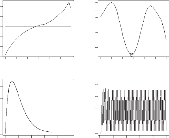
The putative ESS is consistent with the pairwise invasibility analysis but the
elasticity analysis does not indicate that the invasion coefficient is negative for
values different from the putative ESS. In fact, the elasticity analysis suggests that
invasion is highly likely. To view the population dynamics we can simply insert
plot commands into the function POP.DYNAMICS (shown in bold font) and call
this for the optimum a and a value for an invader.
R CODE:
rm(list¼ls()) # Clear memory
DD.FUNCTION <- function(ALPHA,N1,N2) # Density-dependence
function
{
SAME AS IN PREVIOUS
} # End of function
################ POP.DYNAMICS FUNCTION ################
POP.DYNAMICS <- function(ALPHA, Coeff)
{
ALPHA.resident <- ALPHA # Resident value
ALPHA.invader <- ALPHA*Coeff # Invader value
Maxgen1 <- 50 # Nos of generations for resident only
Maxgen2 <- 300 # Nos of generations after invasion
Tot.Gen <- Maxgen1þMaxgen2 # Total number of generations
N.t
Generation
N.tplus1
Elasticity
0 0 20 40 60 80 100
AA
10 15 20 25 30 35 4010 15 20 25 30 35 40
0 200 400 600 800
Population
Invasion.coeff
0 200 400 600 800
–0.003
0.000 0.002 0.004 0.006
–0.001 0.001
200 400 600 800 1,000
Figure 3.17 Elasticity analysis of Scenario 6.
INVASIBILITY ANALYSIS 217
