Richards J.A., Jia X. Remote Sensing Digital Image Analysis: An Introduction
Подождите немного. Документ загружается.


142 6 Multispectral Transformations of Image Data
where m
x
is the data mean in x space. Therefore
Σ
y
= E{(D
t
x − D
t
m
x
)(D
t
x − D
t
m
x
)
t
}
which can be written as
Σ
y
=D
t
E{(x − m
x
)(x − m
x
)
t
}D
2
i.e.
Σ
y
=D
t
Σ
x
D (6.5)
where Σ
x
is the covariance of the pixel data in x space. Since Σ
y
must, by demand,
be diagonal, D can be recognised as the matrix of eigenvectors of Σ
x
, provided D is
an orthogonal matrix. This can be seen from the material presented in Appendix D
dealing with the diagonalization of a matrix. As a result, Σ
y
can then be identified
as the diagonal matrix of eigenvalues of Σ
x
,
Σ
y
=
⎡
⎢
⎢
⎢
⎢
⎣
λ
1
0
0 λ
2
.
.
.
.
.
.
λ
N
⎤
⎥
⎥
⎥
⎥
⎦
where N is the dimensionality of the data. Since Σ
y
is, by definition, a covariance
matrix and is diagonal, its elements will be the variances of the pixel data in the
respective transformed co-ordinates. It is arranged such that λ
1
>λ
2
> ...λ
N
so
that the data exhibits maximum variance in y
1
, the next largest variance in y
2
and so
on, with minimum variance in y
N
.
The principal components transform defined by (6.4) subject to the diagonal
constraint of (6.5) is also known as the Karhunen-Loève or Hotelling transform.
Before proceeding it is of value at this stage to pursue further the examples of
Fig. 6.2, to demonstrate the computational aspects of principal components analysis.
Recall that the original x space covariance matrix for the highly correlated image
data of Fig. 6.2b is
Σ
x
=
1.90 1.10
1.10 1.10
To determine the principal components transformation it is necessary to find the
eigenvalues and eigenvectors of this matrix. The eigenvalues are given by the solution
to the characteristic equation
|Σ
x
− λI |=0, I being the identity matrix.
i.e.
1.90 −λ 1.10
1.10 1.10 − λ
= 0
or λ
2
− 3.0λ + 0.88 = 0
which yields λ = 2.67 and 0.33
2
Since [Aζ ]
t
= ζ
t
A
t
(reversed law of matrices). Note also [Aζ ]
−1
= ζ
−1
A
−1
.
6.1 The Principal Components Transformation 143
As a check on the analysis it may be noted that the sum of the eigenvalues is
equal to the trace of the covariance matrix, which is the sum of its diagonal elements.
The covariance matrix in the appropriate y co-ordinate system (with principal
components as axes) is therefore
Σ
y
=
2.67 0
00.33
Note that the first principal component, as it is called, accounts for 2.67/(2.67 +
0.33) ≡ 89% of the total variance of the data in this particular example. It is now
of interest to find the actual principal components transformation matrix G = D
t
.
Note that this is the transposed matrix of eigenvectors of Σ
x
. Consider first, the
eigenvector corresponding to λ
1
= 2.67. This is the vector solution to the equation
[
Σ
x
− λ
1
I
]
g
1
= 0
with g
1
=
g
11
g
21
≡ d
t
1
for the two dimensional example at hand.
Substituting for Σ
x
and λ
1
gives the pair of equations
−0.77g
11
+1.10g
21
= 0
1.10g
11
−1.57g
21
= 0
which are not independent, since the set is homogeneous. It does have a non-trivial
solution however because the coefficient matrix has a zero determinant. From either
equation it can be seen that
g
11
= 1.43g
21
(6.6)
At this stage either g
11
or g
21
would normally be chosen arbitrarily, and then a
value would be computed for the other. However the resulting matrix G has to be
orthogonal so that G
−1
≡ G
t
. This requires the eigenvectors to be normalised, so
that
g
2
11
+ g
2
21
= 1 (6.7)
This is a second equation that can be solved simultaneously with (6.6) to give
g
1
=
0.82
0.57
In a similar manner it can be shown that the eigenvector corresponding to λ
2
= 0.33
is
g
2
=
−0.57
0.82
The required principal components transformation matrix therefore is
G = D
t
=
0.82 −0.57
0.57 0.82
t
=
0.82 0.57
−0.57 0.82
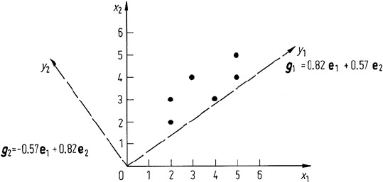
Now consider how these results can be interpreted. First of all, the individual
eigenvectors g
1
and g
2
are vectors which define the principal component axes in
144 6 Multispectral Transformations of Image Data
Fig. 6.4. Principal component axes for the data set of Fig. 6.2b; e
1
and e
2
are horizontal (x
1
)
and vertical (x
2
) direction vectors
terms of the original co-ordinate space. These are shown in Fig. 6.4: it is evident
that the data is uncorrelated in the new axes and that the new axes are a rotation of
the original set. For this reason (even in more than two dimensions) the principal
components transform is classed as a rotational transform.
Secondly, consider the application of the transformation matrix G to find the
positions (i.e., the brightness values) of the pixels in the new uncorrelated co-ordinate
system. Since y = Gx this example gives
y
1
y
2
=
0.82 0.57
−0.57 0.82
x
1
x
2
(6.8)
which is the actual principal components transformation to be applied to the image
data. Thus, for
x =
2
2
,
4
3
,
5
4
,
5
5
,
3
4
,
2
3
we find
y =
2.78
0.50
,
4.99
0.18
,
6.38
0.43
,
6.95
1.25
,
4.74
1.57
,
3.35
1.32
.
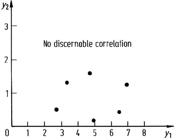
The pixels plotted in y space are shown in Fig. 6.5. Several points are noteworthy.
First, the data exhibits no discernable correlation between the pair of new axes (i.e.,
the principal components). Secondly, most of the data spread is in the direction of the
first principal component. It could be interpreted that this component contains most
of the information in the image. Finally, if the pair of principal component images are
produced by using the y
1
and y
2
component brightness values for the pixels, the first
principal component image will show a high degree of contrast whereas the second
will have limited contrast. By comparison to the first component, the second will
make use of only a few available brightness levels. It will be seen, therefore, to lack
the detail of the former. While this phenomenon may not be particularly evident for a
simple two dimensional example, it is especially noticeable in the fourth component
of a principal component transformed Landsat multispectral scanner image as can
be assessed in Fig. 6.6.
6.1 The Principal Components Transformation 145
Fig. 6.5. Pixel points located in (uncorrelated) principal components space
6.1.3
Examples – Some Practical Considerations
The material presented in Sect. 6.1.2 provides the background and rationale for
the principal components transform. By working through the numerical example in
detail the importance of eigenanalysis of the covariance matrix can be seen. However
when using principal components analysis in practice the user is not involved in this
level of detail. Rather only three steps are necessary, presuming software exists for
implementing each of those steps. These are, first, the assembling of the covariance
matrix of the image to be transformed according to (6.2). Normally, software will be
available for this step, usually in conjunction with the need to generate signatures
for classification as described in Chap. 8. The second step necessary is to determine
the eigenvalues and eigenvectors of the covariance matrix. Either special purpose
software will be available for this or general purpose matrix eigenanalysis routines
can be used. The latter are found in packages such as MATLAB, Mathematica and
Maple. At this stage the eigenvalues are used simply to assess the distribution of data
variance over the respective components. A rapid fall off in the size of the eigenvalues
indicates that the original band description of the image data exhibits a high degree
of correlation and that significant results will be obtained in the transformation to
follow.
The final step is to form the components using the eigenvectors of the covariance
matrix as the weighting coefficients. As seen in (6.4) (noting that G is a transposed
matrix of eigenvectors) and as demonstrated in (6.8), the components of the eigen-
vectors act as coefficients in determining the principal component brightness values
for a pixel as a weighted sum of its brightnesses in the original spectral bands. The
first eigenvector produces the first principal component from the original data, the
second eigenvector gives rise to the second component, and so on.
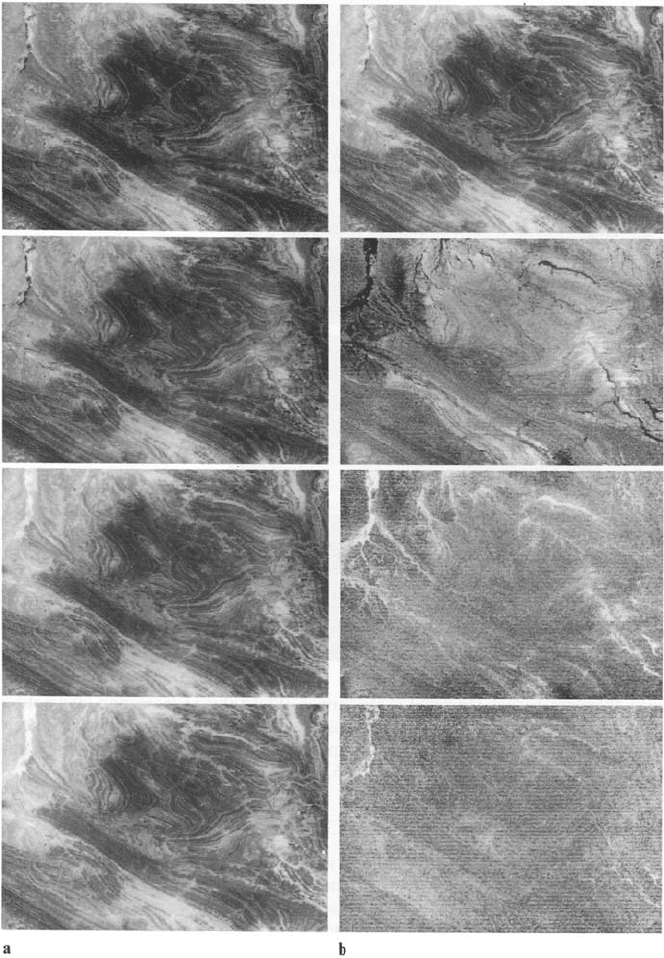
Figure 6.6a shows the four original bands of an image acquired by the Landsat
multispectral scanner for a small image segment in central Australia. The covariance
matrix for this image is
146 6 Multispectral Transformations of Image Data
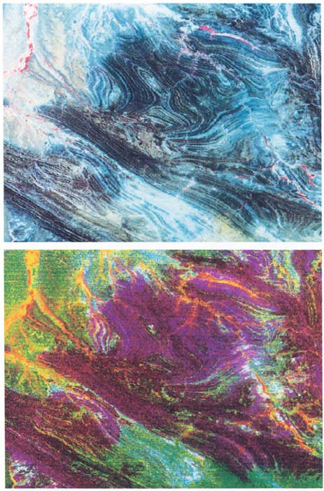
Fig. 6.6. a Four Landsat multispectral scanner bands for the region of Andamooka in central
Australia; b The four principal components of the image segment; c (overleaf) Comparison
of standard false colour composite (band 7 to red, band 5 to green and band 4 to blue) with a
principal component composite (first component to red, second to green and third to blue)
6.1 The Principal Components Transformation 147
Fig. 6.6. c
Σ
x
=
⎡
⎢
⎢
⎣
34.89 55.62 52.87 22.71
55.62 105.95 99.58 43.33
52.87 99.58 104.02 45.80
22.71 43.33 45.80 21.35
⎤
⎥
⎥
⎦
and its eigenvalues and eigenvectors are:
eigenvalues 253.44 7.91 3.96 0.89
eigenvector 0.34 −0.61 0.71 −0.06
components 0.64 −0.40 −0.65 −0.06
(vertically) 0.63 0.57 0.22 0.48
0.28 0.38 0.11 −0
.88
The first principal component image will be expected therefore to contain 95% of
the data variance. By comparison, the variance in the last component is seen to be
148 6 Multispectral Transformations of Image Data
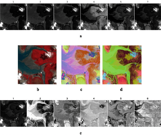
Fig. 6.7. Principal components applied to a highly correlated TM image (without the thermal
band). a Original TM bands; b Colour composite formed from TM bands 4, 3 and 2; c Colour
composite formed from PC3, PC2 and PC1; d Colour composite formed from PC4, PC3 and
PC2; e The full set of principal components.
negligible. It is to be expected that this component will appear almost totally as noise
of low amplitude.
The four principal component images for this example are seen in Fig. 6.6b in
which the information redistribution and compression properties of the transforma-
tion are illustrated. By association with Fig. 6.5 it would be anticipated that the later
components should appear dull and poor in contrast. The high contrasts displayed
are a result of a contrast enhancement applied to the components for the purpose of
display. This serves to highlight the poor signal to noise ratio.
Figure 6.6c shows a comparison of a standard false colour composite formed
from the original Landsat bands and a colour composite formed by displaying the
first principal component as red, the second as green and the third as blue. Owing
to the noise in the second and third components these were smoothed with a 3 × 3
mean value template first.
A second example of the principal components transformation is shown in
Fig. 6.7, this time based on the 6 reflective TM bands for a region in the North-
ern Territory of Australia. The covariance and correlation matrices for the image are:
6.1 The Principal Components Transformation 149
Σ
x
=
⎡
⎢
⎢
⎢
⎢
⎢
⎢
⎣
874.98 550.56 698.00 335.54 858.15 551.21
550.56 363.82 454.79 230.30 558.88 358.38
689.00 454.79 580.63 288.11 747.97 471.72
335.54 230.30 288.11 722.46 742.35 387.61
858.15 558.88 747.97 742.35 1544.70 871.29
551.21 358.38 471.72 387.61 871.29 514.18
⎤
⎥
⎥
⎥
⎥
⎥
⎥
⎦
R
x
=
⎡
⎢
⎢
⎢
⎢
⎢
⎢
⎣
1.00 0.98 0.97 0.42 0.74 0.82
0.98 1.00 0.99 0.45 0.75 0.83
0.97 0.99 1.00 0.44 0.79 0.86
0.42 0.45 0.44 1.00 0.70 0.64
0.74 0.75 0.79 0.70 1.00 0.98
0.82 0.83 0.86 0.64 0.98 1.00
⎤
⎥
⎥
⎥
⎥
⎥
⎥
⎦
By computing the correlation matrix explicitly we can see how likely it is that the
principal components transformation will generate new features quite different from
the recorded measurement vectors. As seen, there is a high degree of correlation
among the bands, so the effect of applying the principal components transformation
should be quite significant. The corresponding eigenvalues and eigenvectors are:
eigenvalues 3727.35 613.34 226.14 23.52 8.16 2.25
eigenvectors first second third fourth fifth sixth
0.433 0.485 −0.307 −0.684 −0.089 0.088
0.282 0.294 −0.218 0.369 0.094
−0.801
0.364 0.347 −0.127 0.627 −0.153 0.561
0.303 −0.673 -0.671 0.018 0.042 0.056
0.615 −0.322 0.562 −0.052 −0.429 −0.129
0.362 −0.047 0.275 −0.026 0.880 0.127
Figure 6.7a shows the original TM bands, while Fig. 6.7e shows the 6 principal
component images. Figure 6.7b shows a colour composite formed by mapping the
original bands 4, 3, and 2 to red, green and blue respectively. Figure 6.7c shows
PC3, PC2 and PC1 mapped to red, green and blue, while Fig. 6.7d shows PC4, PC3
and PC2 mapped to red, green and blue. Interestingly, the PC4, PC3, PC2 colour
composite shows more detail for those ground covers whose spectral responses are
dominant in the visible to near infrared regions, since PC4 (determined by the fourth
eigenvector) is largely a difference image in the visible region. In contrast PC1 is
essentially just a total brightness image, as can be seen from the first eigenvector, so
that it does little to enhance spectral differences.
Notwithstanding the anticipated negligible information content of the last, or last
few, image components resulting from a principal components analysis it is important
to examine all components since often local detail may appear in a later component.
The covariance matrix used to generate the principal component transformation ma-
trix is a global measure of the variability of the original image segment. Abnormal lo-
cal detail therefore may not necessarily be mapped into one of the earlier components
but could just as easily appear later. This is often the case with geological structure.
150 6 Multispectral Transformations of Image Data
6.1.4
The Effect of an Origin Shift
It will be evident that some principal component pixel brightnesses could be negative
owing to the fact that the transformation is a simple axis rotation. Clearly a combi-
nation of positive and negative brightnesses cannot be displayed. Nor can negative
brightness pixels be ignored since their appearance relative to the other pixels in a
component serve to define detail. In practice, the problem with negative values is
accommodated by shifting the origin of the principal components space to yield all
components with positive and thus displayable brightnesses. This has no effect on
the properties of the transformation as can be seen by inserting an origin shift term
in the definition of the covariance matrix in the principal components axes. Define
y
= y − y
0
where y
0
is the position of a new origin. In the new y
co-ordinates
Σ
y
= E{(y
− m
y
)(y
− m
y
)
t
}
Now m
y
= m
y
− y
0
so that
y
− m
y
= y − y
0
− m
y
+ y
0
= y − m
y
.
Thus Σ
y
= Σ
y
– i.e. the origin shift has no influence on the covariance of the data
in the principal components axes, and can be used for convenience in displaying
principal component images.
6.1.5
Application of Principal Components
in Image Enhancement and Display
In constructing a colour display of remotely sensed data only three dimensions of
information can be mapped to the three colour primaries of the display device. For
imagery with more than three bands that means the user must choose the most
appropriate subset of three to use. A less ad hoc means for colour assignment rests
upon performing a principal components transform and assigning the first three
components to the red, green and blue colour primaries.
Examination of a typical set of principal component images for Landsat data,
such as those seen in Fig. 6.6, reveals that there is very little detail in the fourth
component so that, in general, it could be ignored without prejudicing the ability
to extract meaningful information from the scene. A difficulty with principal com-
ponents colour display, however, is that there is no longer a one to one mapping
between sensor wavelength bands and colours. Rather each colour now represents a
linear combination of spectral components, making photointerpretation difficult for
many applications. An exception would be in exploration geology where structural
differences may be enhanced in principal components imagery, there often being
little interest in the meanings of the actual colours.
6.1 The Principal Components Transformation 151
6.1.6
The Taylor Method of Contrast Enhancement
It will be demonstrated below that application of the contrast modification techniques
of Chap. 4 to each of the individual components of a highly correlated vector image
will yield an enhanced image in which certain highly saturated hues are missing.
An interesting contrast stretching procedure which can be used to create a modified
image with good utilisation of the range of available hues rests upon the use of the
principal components transformation. It was developed by Taylor (1973) and has also
been presented by Soha and Schwartz (1978). A more recent and general treatment
has been given by Campbell (1996).
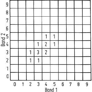
Consider a two dimensional image with the (two dimensional) histogram shown
in Fig. 6.8. As observed the two components are highly correlated as revealed also
from an inspection of the covariance matrix for the image which is
Σ
x
=
0.885 0.616
0.616 0.879
(6.9)
The range of brightness values occupied in the histogram suggests that there is value
in performing a contrast stretch. Suppose a simple linear stretch is decided upon; the
conventional means then for implementing such an enhancement with a multicom-
ponent image is to apply it to each component independently. This requires the one
dimensional histogram for each component to be constructed. These are obtained
by counting the number of pixels with a given brightness value in each component,
irrespective of their brightness in the other component – in other words they are
marginal distributions of the two dimensional distribution. The single dimensional
histograms corresponding to Fig. 6.8 are shown in Fig. 6.9a and the result of applying
linear contrast enhancement to each of these is seen in Fig. 6.9b. The two dimensional
histogram resulting from the contrast stretches applied to the individual components
is shown in Fig. 6.10 wherein it is seen that the correlation between the components
Fig. 6.8. Histogram for a hypothetical two dimensional image showing correlation in its
components. The numbers indicated on the bars (out of page) are the counts
