Pump Handbook by Igor J. Karassik, Joseph P. Messina, Paul Cooper, Charles C. Heald

Подождите немного. Документ загружается.

9.333

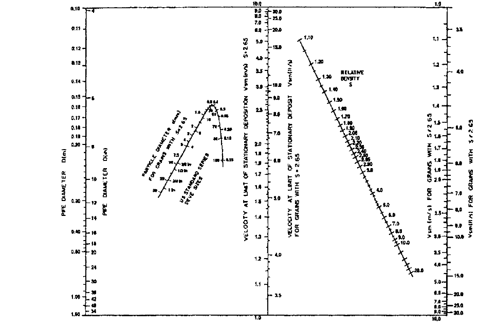
FIGURE 6 Nomographic chart for maximum velocity at limit of stationary deposition (from

Wilson, 1979).

9.334 CHAPTER NINE

virtually unaffected by a variation of the particle diameter between 0.015 and 0.04 in. (0.4

and 1.0 mm). However, the right limb of the particle-diameter curve shows greatly

increased sensitivity, so that a change in d from 0.006 to 0.008 in. (0.15 to 0.20 mm) alters

by more than 25 percent.

It is found that a change of the relative density does not influence the form of the rela-

tion shown on Figure 6, but does require its “recalibration.” This is accomplished graphi-

cally by using the inclined relative-density axis on the right-hand side of the figure. To

illustrate the use of the right-hand panel of Figure 6, consider again the pipe 12 inches

(0.30 m) in diameter, now carrying particles with a diameter of 0.004 in. (1.0 mm) and rel-

ative density 1.50. With 0.004 in. (1.0 mm) entered on the particle scale, a straight line

joining it to the pipe diameter can be projected to the central axis of the figure, showing

that V

is 11.5 ft/s (3.5 m/s) for the equivalent sand size. In order to correct this for the rel-

ative density of 1.50, the latter value is entered on the sloping axis on the right-hand side

of the figure and joined by straight-edge to the point just found on the central axis (11.5

ft/s or 3.5 m/s). The projection of this line to the vertical axis on the right of the figure gives

the adjusted value of the maximum deposition velocity, approximately 6 ft/s (1.9 m/s).

Particles that differ in density from sands may also have different values of other prop-

erties, including the solids fraction in the deposit and the mechanical friction coefficient

between the particles and the pipe. The values of these quantities that were employed in

the computer program, and hence are reflected in the nomographic chart, apply to sands

but not necessarily to other materials.Therefore the values of V

determined from Figure

6 for materials other than sands must be treated as somewhat less accurate than values

for sand. However, both the solids fraction in the bed and the particle-pipe mechanical fric-

tion coefficient occur in the computer program only as multiples of the submerged relative

density of the particles, and it is found that any change in these quantities merely gives

rise to a multiplicative factor which must be applied to the values of V

obtained from the

figure. This permits calibration of the output of the nomographic chart from a few pilot-

plant tests with the material of interest.

The particle diameter scale of Figure 6 has not been extended below 0.006 in. (0.15

mm) since smaller particles tend to be influenced by mechanisms not included in the

mathematical model on which the nomogram is based. As shown by Thomas (1979) the

viscous sublayer can have a significant effect, and all particles which are small enough

to be completely embedded in this sublayer will behave in a fashion which is no longer

dependent on particle diameter. In this limiting case certain simplifications can be made

in the mathematical model. Thomas found that these lead to a simple expression for the

shear velocity at the limit of stationary deposition, and on employing a power law approx-

imation for the friction factor, he then obtained a corresponding expression for V

(18)

Here n represents the kinematic viscosity of the carrier fluid (i.e. m/r), and the coefficient

of 9.0 applies in any consistent system of units.This equation gives the minimum value of

deposition velocity for small particles, assuming turbulent flow.

For cases where the interfacial friction sets up a sheared layer several grain diameters

in thickness, a new analysis has been developed (Wilson, 1988;Wilson & Nnadi, 1990). For

large pipes, and particles near the Murphian size, this new analysis shows that the parti-

cle size no longer influences V

directly. In such cases the value of V

is less than that

predicted by Figure 6, a point which is in accord with experimental evidence. It is then nec-

essary to obtain the value of V

from the new analysis of Interfacial friction, for compar-

ison with the value from the nomographic chart.

When the parameters in the new analysis are given values typical for sands, it is found

that the dimensionless maximum deposition velocity (i.e. the Durand deposition variable)

depends only on the fluid friction factor for the portion of the pipe wall above the deposit.

A power-law approximation gives an appropriate fit function for this effect, i.e.

(19)

max

22gD1S

 S

 a

0.018

0.13

 9.03gn1S

 S

0.37

1D>v2

0.11

9.16.1 HYDRAULIC TRANSPORT OF SOLIDS 9.335

where f

is the friction factor for fluid alone. If the value of V

found from the nomo-

graphic chart exceeds the value of (V

)

max

from Eq. 19 the latter value should be used

for V

Fully Stratified Coarse-Particle Transport Fully-stratified flow occurs where almost

all of the particles travel as contact load (i.e. fluid suspension is ineffective). The ratio of

particle diameter to pipe diameter is of major importance in determining the presence of

this flow type, which does not normally occur for d/D ratios less than 0.015. Fully-stratified

flow is less likely if the particles are broadly graded, especially if there is a significant

homogeneous fraction (i.e. a significant fraction of particles smaller than 200 mesh/75

mm). Calculations made for narrow-graded slurries with water as a carrier fluid indicate

fully-stratified behavior for values of d/D above 0.018.

Although the actual relationship of the detailed force-balance analysis cannot be

expressed in closed form, simple approximating functions can be fitted to match the out-

put of the detailed model. Wilson & Addie (1995) proposed the following expression for

approximating fully-stratified flow:

(20)

The ratio on the left hand side of this equation is the same as that used by Newitt et

al. (1955), and the right hand side shows the decrease of this ratio with increasing V

The coefficient B¿ has a value of 1.0 for angular particles, and decreases with the degree of

rounding. For typical cases the suggested default value is 0.75. As fully-stratified flow has

higher energy consumption than other flow types, Eq. 20 can be thought of as represent-

ing the upper limit of excess pressure gradient (i.e. solids effect). Heterogeneous slurry

flows, which are covered in the following section, will generally display smaller values of

the solids effect.

Another type of stratified flow that may be encountered is flow above a stationary bed

of solids. This type of operation is generally uneconomic, and thus is seldom a deliberate

design choice, but it is sometimes found in existing pipelines. Flow over a stationary bed

has been studied experimentally, and analyzed by a computer model (Nnadi & Wilson,

1992; Pugh, 1995). For most cases of this type of flow encountered in pipelines the follow-

ing rough approximation to the computer output may be sufficient. It is based on particles

near the “Murphian” size, which tend to be disproportionately represented in stationary

deposits:

(21)

Pressure Gradients for Partially-Stratified Flow As mentioned previously, two meth-

ods of support are significant in partially-stratified flows: turbulent suspension and gran-

ular contact. For turbulent suspension the eddies can carry the particles with no

significant additional energy consumption, but granular contacts set up Coulombic fric-

tion forces which must be overcome by an additional “solids effect” pressure gradient, rep-

resented by (i

 i

) where i

(or i

) is the hydraulic gradient for fluid only. In many cases

this solids effect varies with the submerged weight of solids, i.e. with (S

 S

where S

is the relative density of the fluid (1.0 for water) and C

is the volumetric delivered con-

centration. The quantity (S

 S

can also be expressed as (S

 S

) where S

is the

relative density of the mixture. The relative solids effect, written (i

 i

)/(S

 S

), can

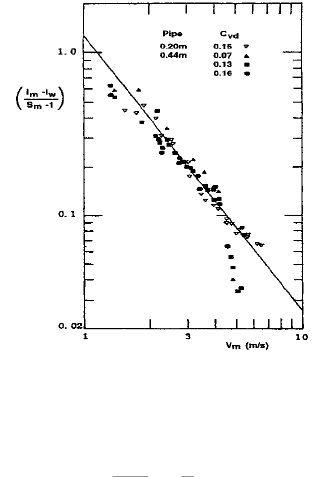
be obtained from pipe-loop testing. Typical results for partially-stratified flow are shown

on Figure 7 for various concentrations of sand with d

of 0.016 in. (0.42 mm). The rela-

tive solids effect drops with increasing mean velocity V

, which in turn produces increased

turbulent fluctuating velocities, implying that a larger fraction of particles will be sus-

pended by turbulence. The straight fit line shown on the logarithmic coordinates of Fig-

ure 7 indicates that the relation can be approximated by a power law. (Other formulations

have also been proposed, see for example Shook & Roco, 1992 and Gillies et al., 1991.)

 0.321S

 12

1.05

0.6

22gD

0.1

 i

 12

 B¿ a

0.55V

0.25

9.336 CHAPTER NINE

FIGURE 7 Behavior of masonry-sand slurry (d

= 0.42 mm) in pipes of two sizes (after Clift et al., 1983). [m 

3.28 = ft; m/s  3.28 = ft/s]

In addition to the slope parameter (denoted by M) a power law requires a central-value

parameter, denoted here by V

. Conceptually, this represents the value of V

at which half

the mass of solids is supported by granular contact and half by fluid suspension. From a

practical standpoint it is necessary to match this point with a specific value of (i



)/(S

 S

). The mechanics of the situation were discussed by Wilson et al. (1997) who pro-

posed a value of 0.22 and showed that this is suppoted by experimental data. The result-

ing equation is

(22)

If test data are available, M and V

can be obtained directly from the results. For

example consider the data of Figure 7 in the 8 in. (0.20 m) pipe. In calculating the ratio

 i

)/(S

 1), the clear water gradient i

has been used to approximate i

, and S

is S

 i

 S

 0.22 a

M

9.16.1 HYDRAULIC TRANSPORT OF SOLIDS 9.337

i.e. 1.0. The value of i

was calculated from the Darcy-Weisbach formula using the friction

factor f

 0.013 measured previously for flows of water in this pipe.The plotted points fall

on an essentially straight line on Figure 7. This behavior corresponds to Eq. 22. The slope

of the line gives M  1.7, which is typical for slurries with narrow particle grading. The

point on the line where (i

 i

)/(S

 1)  0.22 gives V

, which is approximately 9 ft/s

(2.8 m/s).

With V

and M obtained for the 8 in. (0.20 m) pipe, scale-up to a larger pipe diameter

can be carried out. The larger diameter of 18 in. (0.44 mm) has been selected because data

are available with the same sand in this larger pipe (Clift et al., 1982) and thus the scaled-

up results can be verified directly. In fact, as seen on Figure 7, the fit line for the larger pipe

coincides with that for the smaller pipe in this instance. In this case the clear-water friction

factor f

was found to be the same for both pipes and in both pipes the particle size d was

a small fraction of the pipe diameter. It has been found that V

should vary with (8/f

)

1/2

;it

should also depend on the diameter ratio d/D (Wilson & Watt, 1974; Wilson et al., 1997).

These factors can be incorporated in the scale-up procedure, which involves preparing

curves of i

versus V

for various values of C

in the larger pipe, the relation for each line

of constant C

being expressed as

(23)

It is typical to find a moderate decrease in f

with increasing pipe size, which produces a

small increase in V

. Increases in D have the opposite effect, but for small ratios of d/D,

as is the case for the data of Figure 7, this effect is not significant.

Other problems arise when pipeline experiments have not been carried out with the

particular slurry of interest. In many cases of practical importance, information on the size

and grading of the material to be pumped is limited, but estimates of the solids effect must

be made. For example, consider the case of an ore that is to be crushed and then trans-

ported by pipeline. At the initial stage of the design there may be no adequate sample of

the crushed ore, but estimates of the effect of the solids on the head loss must be made for

feasibility studies, preliminary designs and cost estimates, and even for justifying the

expenses of laboratory or pilot-plant testing.

To estimate the solids effect, two parameters are required: the power M and the veloc-

ity V

. The value of M has a lower limit of 0.25 (for fully-stratified flow) and approaches

1.7 for slurries with narrow particle grading. If only a rough idea of the grading is avail-

able, it may be adequate to use the following approximation, which requires only an esti-

mate of the particle diameter ratio d

is the mass-median particle diameter and

is the diameter for which 85% by mass of the particles are smaller). Using this evalu-

ation, the approximation for M is written

(24)

Here /n is the natural logarithm. Also, M should not be allowed to exceed 1.7 or fall

below 0.25.

The next step is to obtain a commensurate approximation for V

(Wilson et al., 1997).

This formula reads

(25)

Here d

is in mm. The coefficient 3.93 applies for velocities in m/s; for velocities in ft/s this

coefficient becomes 12.9. With sand-weight solids (S

 1) equals 1.65 and the bracketed

portion of Eq. 25 equals 1.00. The value of V

obtained from Eq. 25 is substituted into Eq.

22 to obtain the solids effect (i

 i

), where i

is the gradient for an equal flow of water.

Note, Eq. 25 is only applicable for 0.006 in  d

 0.055 in (0.15 mm  d

 1.4 mm). For

larger particles the value of V

given by Eq. 25 should be multiplied by cosh(60d

/D).

Remarks on Complex Slurry Flows In the introduction to this section, it was men-

tioned that slurry flows can be divided into three types on the basis of mechanisms of par-

ticle support. These types are homogeneous, partially-stratified and fully stratified, and

 3.93d

0.35

31S

 12>1.654

0.45

M  3/n1d

1



2gD

 0.221S

 12V

M

9.338 CHAPTER NINE

the applicable methods of analysis for these flows have been outlined in the appropriate

preceding sections. Quite often, the particle grading curve is sufficiently broad to span two

of the flow types, or even all three. This gives rise to complex slurry flows. The larger par-

ticles, which would settle readily in water, often receive considerable support from the

smaller particles and the carrier fluid, promoting efficient transport. A complete analysis

of such flows is not yet available, but it is hoped that the following remarks will aid the

design engineer.

Whenever some coarse particles settle, they form contact load. As shown in earlier sec-

tions of this chapter, this has an effect on pressure drop which is quite different from that

of particles suspended by the fluid. The contact-load effect, analyzed previously for the

case of a Newtonian carrier fluid, must eventually be combined with the scaling laws for

non-Newtonian fluids presented in an earlier part of this chapter. As laminar flows which

have significant particle settling are usually avoided in design, only turbulent flows will

be considered here.

Maciejewski et al. (1993) compared large-diameter transportation of coarse particles

of about 4 in. (100 mm) in clay suspensions and in oil-sand tailings slurries (particle size

below 0.03 in./0.8 mm). They found that the sand slurry was more effective as a trans-

port medium than a viscous, homogeneous clay slurry. The important role of particles

with sizes of 0.004 to 0.020 in. (0.1 to 0.5 mm) in reducing friction was further shown in

studies by Sundqvist et al. (1996a, 1996b) for products with d

of 0.024 to 0.027 in. (0.6

to 0.7 mm) and various size distributions, with maximum sizes of up to 6 in. (150 mm).

In studying the behavior of complex slurries like these, it is logical to begin by dividing

the total concentration of solids C

into three components, each associated with a support

mechanism. Thus C

stands for homogeneous, C

for partly stratified (the “middlings”)

and C

for the coarse fully stratified particles (the “clunkers”). On the basis outlined pre-

viously the particle size of 200 mesh (75 mm) separates C

and C

and the size 0.018D sep-

arates C

and C

. This point is best illustrated by an example. Take S

 2.65; and a

concentration of 30% by volume (C

 0.30). From the solids grading curve, suppose that

20% of the total is slimes, 50% middlings and 30% clunkers. Thus, the concentration of

slimes in the slurry is (0.30)(0.20)  0.06, and similarly 0.15 and 0.09 for middlings and

clunkers, respectively. The equivalent fluid based on the slimes has specific gravity S

 1

 (S

 1)C

 1  (1.65)(0.06)  1.099 and that for the combined slimes and middlings

is S

hmi

 1  (1.65)(.21)  1.347. Thus, for the middlings the specific gravity difference

between solids and carrier fluid is (2.650  1.099)  1.551 (rather than 1.650). For the

clunkers, the equivalent difference is (2.650  1.347)  1.303.

The homogeneous fraction now forms the carrier fluid for the rest of the slurry, and its

hydraulic gradient i

replaces i

in equations like Eq. 20 and Eq. 22. These are used to

determine the solids effect for middlings and clunkers, which may be written i

and i

The gradient for the mixture i

represents the sum of i

and the solids effects for the mid-

dlings and the clunkers, i.e.

(26)

The homogeneous gradient i

is based on appropriate equivalent-fluid or non-Newtonian

calculations, as given previously. For the middlings, i

is effectively equivalent to (i



) in Eq. 22, when applied to the middlings only, giving

(27)

Here, S

is the relative density of the homogeneous “carrier fluid” component (1.099 for

the example just introduced). The evaluation of M and V

will be mentioned in the fol-

lowing text.

For the clunkers, i

is based on Eq. 20, except that the carrier fluid for the clunkers

now includes both the homogeneous portion and the middlings, with a relative density

written S

hmi

(1.347 for the example). The carrier fluid will also have an effect on the coef-

ficient which will now be written B– instead of B¿ (the evaluation of B– will be mentioned

next). The relation for i

¢i

 C

 S

20.22 a

M

 i

 ¢i

9.16.1 HYDRAULIC TRANSPORT OF SOLIDS 9.339

(28)

For coarse solids only, it was suggested above that the parameter B¿ in Eq. 20 should have

a default value of 0.75. When considerable fractions of middlings are found, B¿ must be

reduced to give B–. As it is expected that the reduction is associated with density differ-

ences, the appropriate variable would appear to be the weight concentration, C

, of fines

plus middlings, i.e. C

whmi

(for the example C

whmi

 0.372). Thus

(29)

where j is a coefficient with a proposed default value of unity.

Another point concerns the evaluation of V

and M for the middlings. The methods of

Eqs. 24 and 25 are basically applicable but d

and d

must now refer to the middlings

fraction only, rather than the whole grading curve. For very broad well-distributed grad-

ings the middlings will simply be a slice between 0.003 in. (0.075 mm) and 0.018D. Here

it may be possible to assume that d

is the geometric mean of the two diameter limits (e.g.

0.025 in. for D  1 ft or 0.64 mm for D  0.305 m). For this case a default value of about

1.0 might be appropriate for M. V

will be influenced by the rheological properties of the

homogeneous fraction, which will influence the fall velocity of the middling particles, thus

enhancing suspension. An initial approach is to consider the homogeneous part of the

slurry to act as a Newtonian fluid with effective viscosity significantly higher than that of

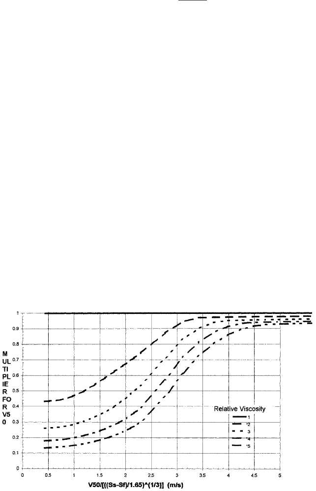
water. The effect of enhanced viscosity on V

is of the form shown on Figure 8. On this fig-

ure the value of V

based on water viscosity is entered on the abscissa (corrected for rela-

tive density of solids if different from 2.65). The various curves are for different m

, the

ratio of viscosity to that of water at 70°F (20°C). The multiplier read from the ordinate can

be applied to the V

value for water to estimate V

in the higher-viscosity carrier fluid.

EXAMPLE

2 This example pertains to fully-stratified flow of coarse magnetite particles

(d  1 in. or 25 mm). Because of their high relative density (S

 4.4) these particles are

to be used as ballast for an offshore drilling rig.The magnetite will be transferred from

ore carriers to the rig by a dredge pipeline with internal diameter 19.7 in. (0.500 m).

a. Find the deposition limit in this line, V

. Figure 6 is entered with the pipe

diameter (on the left axis) and the particle diameter (on the demi McDonald).

B''  B'11  jC

whmi

¢i

 C

 S

hmi

2B– a

0.55V

0.25

FIGURE 8 Variation of V

with viscosity

9.340 CHAPTER NINE

Projection to the central axis gives V

 8.7 ft/s (2.65 m/s) for sand-weight

material. This number is joined to the relative density S (i.e. S

) of 4.4 on the

sloping axis and projected to the right-hand axis to give V

 13 ft/s (4.0 m/s) for

the magnetite.

b. Find the hydraulic gradient i

for a volumetric solids concentration of 0.10 and a

throughput velocity V

 16.4 ft/s (5.0 m/s). Assume rather angular material with

B¿  0.9. The first step is to calculate the clear-water friction gradient of i

. Using

 0.013, i

is given by or 0.033 (height of water per length of pipe).

To this must be added (i

 i

), which Eq. 20 gives as (S

 1)B¿(V

/0.55V

)

0.25

The quantity (S

 1) equals C

 1) i.e. (0.10)(3.4)  0.34. B¿ has been taken as

0.9 and the ratio (V

/0.55V

) equals 2.27, giving (i

 i

)  0.250 and i

 0.28,

i.e. 28 ft of water per 100 ft of line or 0.28 m of water per m of line. Very large gra-

dients like this, which have been verified in prototype-scale testing, show why

fully-stratified flow is only of interest for short-haul applications.

EXAMPLE 3

a. Suppose that the magnetite of the previous example has been ground to give d

 0.008 in. (0.20 mm) and d

 0.012 in. (0.30 mm). As in the previous example,

D  1.64 ft (0.50 m) and V

 16.4 ft/s (5.0 m/s). In this case the volumetric

concentration C

 0.20. Find the V

and the hydraulic gradient i

is found as in the previous example.The pipe size is joined to the particle size

of 0.008 in. (0.20 mm) and projected to the central axis to give the deposition

velocity for sand-weight solids. Solids specific gravity is entered on the sloping

line, and projected to the right-hand axis to give V

 14.4 ft/s (4.4 m/s). As in

the previous example this is less than the proposed operating velocity, which is

satisfactory.

The flow of this slurry will be partially stratified, and from Eq. 24, M 

[/n(0.30/0.20)]

1

 2.5. However, the maximum limit of M is 1.70, which will be

used here. From Eq. 25,

For this value of V

, with M  1.7 and V

 16.4 ft/s (5.0 m/s), the right hand

side of Eq. 22 becomes 0.098. (S

 1) equals (S

 1)(C

)  (3.40)(0.2)  0.68.

Hence

 i

 (0.68)(0.098), and with i

of 0.033 (found in Example 2) i

is found to be

0.100 (ft water per ft or m water/m). Note that this gradient is only about one-

third that for the coarse particles of the previous example, despite the fact that

the solids concentration (and the tonnage transported) is twice as much.

b. As in part (a) but with d

 0.016 in. (0.40 mm). The power M is re-evaluated as

M  [/n(0.40/0.20)]

1

 1.44. For the unchanged values of V

and V

, the right-

hand side of Eq. 22 becomes 0.110 and i

equals 0.033  0.68 (.110) or 0.108 (ft

water/ft or m water/m).

c. As in part (a) but assume that there is a fine-particle fraction that increases the

viscosity of the homogeneous component to 4 times that of water. From part (a),

M  1.70 and V

 10 ft/s (3.1 m/s) in water. Adjusting for the density difference

from the sand-water case gives the abscissa of Figure 8 as 3.1/(3.40/1.65)

0.33

i.e. 7.88

ft/s (2.4 m/s). With this abscissa and a relative viscosity of 4, Figure 8 gives a mul-

tiple of 0.42, for a revised estimate of V

as (0.42)(3.1)  4.3 ft/s (1.3 m/s). Thus the

right/hand side of Eq. 22 beocmes 0.022, and i

 .033  0.015 or 0.048 (ft water/ft

or m water/m). This revised estimate is only about one-half the value of 0.100

obtained in part (a) for pure water as the carrier fluid.

 3.9310.202

0.35

3.40

1.65

0.45

 3.1 m>s 110 ft>s2

0.013V

>2gD

9.16.1 HYDRAULIC TRANSPORT OF SOLIDS 9.341

OTHER FACTORS ____________________________________________________

Vertical Flows

For industrial application of vertical transportation of a solid-liquid mix-

ture in a pipe, the operating velocity must be sufficient to maintain a continuous flow of

solids at the discharge end. However, unnecessarily high velocity causes excessive pipe

wear and energy losses. The appropriate operating velocity depends on the settling con-

ditions of the solids, indicating that size, density, and concentration of particles are key

parameters in the hydraulic design of a vertical particle-fluid transportation system.

Many experimental studies have been made of vertical slurry transport. For example,

Sellgren (1979) used a pilot-scale facility with a centrifugal pump to investigate important

design parameters for ores and industrial minerals taken from in-plant crushing and

milling. The results of these experiments are summarized in the following paragraphs.

It is suggested that the allowable minimum mixture velocity be based on the settling

velocity of the largest particles in still water multiplied by a factor of 4 or 5. Provided the

velocity exceeds this value, then in most industrial applications, with volumetric concen-

trations of 15

—

30%, the corresponding pressure requirement in the vertical system can be

determined by the equivalent-fluid model. As noted in connecetion with Eq. 5, this model

is based on the density of the slurry and the friction factor for water. Applied to vertical

flow, it gives

(30)

Here p is the pressure required, S

is the relative density of the slurry, z is the length of

vertical pipe, and V

all

is the allowable minimum mixture velocity, approximately four times

the settling velocity of the largest particle.

The settling velocity in still water of industrially-crushed mineral particles is normally

reduced significantly compared to smooth spheres of corresponding size.Tests have shown

that, on average the settling velocity for particles in the range of 0.04 in. to 1.2 in. (1 mm

to 30 mm) is reduced approximately 50%. Therefore, the criterion previously given for the

minimum allowable velocity could alternatively be formulated as: V

all

is twice the settling

velocity of a smooth sphere of the same size as the largest particles.

Within the constraints previously discussed, systems operate under conditions where

the effect of relative velocity between the components appears to be negligible. The maxi-

mum particle sizes considered are in the range of 0.04 in. to 1.2 in. (1 mm to 30 mm) in

pipe diameters of 4 to 12 in. (0.1 m to 0.3 m). With larger particle sizes (up to 4 to 6 in./100

to 150 mm) and low concentrations, the relative velocity between the components becomes

significant. Boundary-layer transitional effects may also introduce certain instabilities

that must be carefully evaluated in long vertical risers. Particles larger than one-fifth the

pipe diameter can promote slugging instability in vertical hoisting, and particles larger

than one-third the pipe diameter may jam the pipe and should be avoided.

EXAMPLE 4 Centrifual slurry pumps are used to pump a sand slurry (d

 0.06 in./1.5

mm) out of a quarry. The pipe is vertical with a length of 328 ft. (100 m) and a diame-

ter of 4 in. (0.10 m). Tests have shown that the settling velocity of the largest particles

is approximately 1.5 ft/s (0.45 m/s). Select the operating velocity and calculate the head

requirement in meters of slurry.

Solution Following the guidelines previously given, the velocity V

all

is four times 0.45, i.e.

6 ft/s (1.8 m/s). At this velocity, is 0.54 ft (0.165 m). With the friction factor f

taken

as 0.016 for smooth-pipe conditions (see Figure 2), the head is obtained from Eq. 30 as

in USCS units or 336.5 S

in ft of water.

328c1 

0.01610.5412

3.94>12

d 336.5 ft of slurry

>2g

p  r

za1 

2gD

b1for V

7 V

all

9.342 CHAPTER NINE

In SI units the calculation becomes

or 102.6 S

in meters of water.

Inclined Flows Lengths of pipe with an adverse slope often form part of pipelines trans-

porting solids. Compared to the horizontal case, flow up an incline tends to require higher

throughput velocities in order to avoid deposition. This is of greatest significance for

coarse-particle flow.

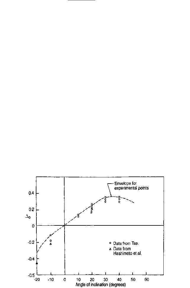
In an experimental investigation carried out by Wilson & Tse (1984), four particle sizes

between 0.04 and 0.24 in. (1 and 6 mm) were tested in a pipe at angles of inclination up to

40 degrees from the horizontal. It was found that the velocity at the limit of deposition ini-

tially increases with the angle of upward inclination, u, reaching a maximum when this

angle is about 30 degrees. For the materials tested this maximum velocity was approxi-

mately 50 percent larger than that required to move a deposit in a horizontal pipe. This

large difference is clearly a matter of importance for both design and operation of pipelines

with inclined sections.

As indicated schematically on Figure 1, V

marks the lower end of the range of desir-

able operating velocities for a pipeline. For purposes of comparison, it is appropriate to rep-

resent the deposition limit for inclined flow in terms of the dimensionless velocity, or

Durand number, V

/[2g(S

 1)D]

1/2

. The difference between the Durand number for

inclined flow and that for horizontal flow, D, is plotted against u on Figure 9.

For the effect of pipe inclination on friction loss, the following widely-used formula by

Worster & Denny (1955) may be employed for heterogeneous flows and homogeneous flows

in which the hold-up effects are small. Their approach, based on water as the carrier fluid,

deals with the extra pressure gradient (i(u), expressed in height of water per length of pipe)

beyond that for pumping water alone. For horizontal flow, this extra gradient is simply the

solids effect (i

 i

), which may be written i(0). Worster and Denny’s formula states that

(31)

For highly stratified flows, Eq. 31 underestimates the losses. For further information see,

for example, Wilson et al. (1997).

¢i1u2 ¢i102cos u  1S

 12C

sin u

100c1 

0.01610.1652

0.1

d 102.6 m of slurry

FIGURE 9 Effect of angle of inclination on Durand deposition parameter (after Wilson and Tse, 1984)

Pump Handbook by Igor J. Karassik, Joseph P. Messina, Paul Cooper, Charles C. Heald - 3rd edition

Подождите немного. Документ загружается.