Prinz H. Numerical Methods for the Life Scientist
Подождите немного. Документ загружается.

The result of the typing should be a plot giving a parabola, a text within the plot,
Hallo as a title, and a label “World” for the x-axis. If all these commands are
understood, this tutorial has been finished successfully.
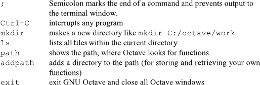
Some commands which may also be useful:
4.8 Recommended Literature for Octave/MATLAB
This will conclude a first elementary introduction to octave. There is extensive
literature and helpful information to be found abundantly in the Internet. Both GNU
Octave and MATLAB are living languages, which present their current
developments in the Internet, so that written textbooks may seem to be obsolete.
There are noteworthy exceptions: Cleve Moler has written an introductory course
on numerical methods [3], which gives the necessary background for numerical
methods applied here. Individual chapters can be downloaded from Mathworks.
com [ 4 ]. MATLAB comes with extensive documentation and help functions. For
GNU octave, its manual [5] is a useful piece of hardware. It gives an overview and
can be used as an excellent reference for each command. It is a useful investment,
although its contents are shown directly in the Octave terminal window with the
command doc. There is a very active GNU Octave community, so that there are
more than 326,000 Google h its for “Octave Tutorial”. Some of these seem to be
particularly useful [6–8], and most tutorials cover MATLAB as well. MATLAB is
at least as popular as Octave, with 571,000 Google hits for “MATLAB Tutorial”.
Tutorials may be available in any spoken language worldwide.
Octave and MATLAB have a broad application spectrum, mainly focused on
science and engineering. Only a few of these features are required for the calcula-
tion of reaction schemes. They are introduced one by one as they come along to
solve practical problems.
References
1. http://www.gnu.org/software/octave/license.html
2. http://en.wikibooks.org/wiki/MATLAB_Programming/Differences_between_Octave_and_MA
TLAB
40 4 Getting Started with Octave
3. Moler C (2010) Numerical computing with MATLAB. Society for Industrial Mathematics,
Philadelphia, PA
4. http://www.mathworks.com/moler/chapters.html
5. Eaton JW, Bateman D, Hauberg S (2008) GNU octave manual version 3. Network Theory Ltd,
London
6. http://smilodon.berkeley.edu/octavetut.pdf
7. http://en.wikibooks.org/wiki/Octave_Programming_Tutorial
8. http://srl.informatik.uni-freiburg.de/downloadsdir/Octave-Matlab-Tutorial.pdf
References 41
.
Chapter 5
Equilibrium Binding
Binding equilibria of n compounds can be calculated from n equations of n
unknowns. These are solved numerically with the Octave /MATLAB subroutine
fsolve. Writing program code for this task is introduced step by step. The output
of all programs is given in a graphic format so that binding mechanisms of
increasing complexity can be visualized. Allosteric interactions of subunits and
multiple allosteric interactions at one target molecule are calculated as practical
examples. At the end of this chapter , the reader should be able to calculate
equilibrium binding for any reaction scheme involving any number of ligands,
inhibitors and binding sites.
5.1 Solving Nonlinear Equations for Equilibrium Binding
Sections 2.2 and 2.3 describe the sets of nonlinear equations derived from equilib-
rium-binding schemes. In Octave and MATLAB, these equations are solved with the
function fsolve, which in turn is based on the MINIPACK subroutine hybrid [1].
MATLAB users must obtain the “Optimization toolbox,” which includes fsolve.
The set of equations to be solved has to be written as an array of n equations with
n unknowns. In Octave/MATLAB, such an array is treated as a vector, and the set of
equations can be written as a vector function
FðxÞ¼0 (5.1)
F and x are vectors of the same size. The function fsolve requires an initial
estimate for the unknowns, a vector xo. It then calculates the set of equations as F
(x0). The result will not be zero, but fsolve varies the unknowns x in several steps
until (5.1) is solv ed within the required mathematical precision.
This general strategy has to be illustrated with an example; reversible binding to
one site leads to (2.16) and (2.17) for equilibrium binding. These equations can be
re-written as elements of the function (5.1):
H. Prinz, Numerical Methods for the Life Scientist,
DOI 10.1007/978-3-642-20820-1_5,
#
Springer-Verlag Berlin Heidelberg 2011
43
F(1) ¼ x(1) þ x(1) x(2)/KD1 R0 ¼ 0 (5.2)
F(2) ¼ x(2) þ x(1) x(2)/KD1 L0 ¼ 0 (5.3)
Remember, x(i) denotes the ith element of the vector of unknowns x, with
x(1) ¼ [R] and x(2) ¼ [L]. Likewise, the initial estimates will also be defined as
one vector x0. When R0 and L0 are similar, the free concentrations are estimated to
be half of the total concentrations:
x0ð1Þ¼0:5 R0 (5.4)
x0ð2Þ¼0:5 L0 (5.5)
Note: When the ligand concentration is much larger than the receptor concen-
tration, equation (5.6) becomes a better estimate for the free ligand concentration:
L0 >> R0 : x0ð2Þ¼L0 0:5 R0 (5.6)
Having explained the basic concept of iterative techniques used in fsolve, this
function can now be applied in a sample program. The function fsolve is called with
the statement: x ¼ fsolve('name',x0), where 'name' is the name of the
function for the set of (5.2) and (5.3). x0 and x are column vectors of the same
length. Remember, Octave and MATLAB are matrix-oriented languages, and all
variables may be matrices, vectors or scalars.
5.2 Equilibrium Binding to One Site (EQ1.m)
The first sample program is EQ1.m, a program which calculates reversible binding
to one site with analytical and numeric methods. The central function, called from
fsolve, is called EQ1F.m. It is stored with this name in the octave work directory.
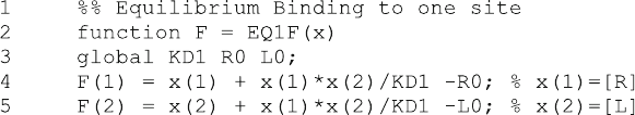
It mainly contains (5.2) and (5.3) written in Octave code.
The first line is merely a description of the function. It is written as a “comment.”
Comments are defined as lines beginning with the percent sign %. In MATLAB, two
of these signs (line 1) define the beginning of a program section. The % sign may not
only appear at the beginning, as illustrated in lines 4 and 5. In this case, the
comment begins at the % sign and ends at the end of the line. The function
44 5 Equilibrium Binding
statement (line 2) defines the name of the function (EQ1F). The function names in
this textbook are derived from the names of the main program, suppl emented by the
letter F. The name of a function must be the same as the name of the file in which it
is stored (EQ1F.m). The letter F in line 2 defines the variable name which is
returned from the function. The components of the vector F are calculated in lines 4
and 5. They correspond to (5.2) and (5.3). The global statement in line 3 allows
data exchange between the function and the main program.
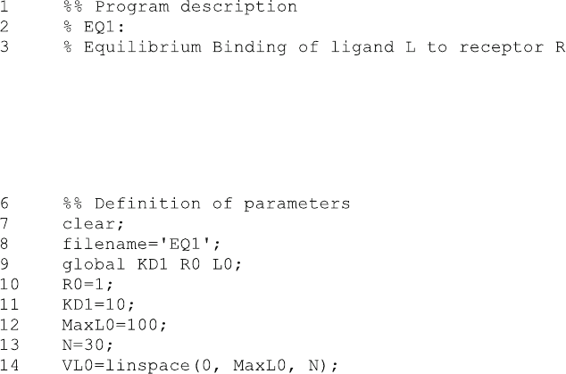
The main program (EQ1.m) also begins with a short description given as
comment lines.
The next section of EQ1.m is the definition of all relevant parameters. It is
usually a good idea to define parameters at the beginning of a program. Computer
code is read from top to bottom so that any variable has to be defined before it is
used. When all variables are defined together in consecutive lines, it is easy to
identify them for debugging or modifying the program.
Clear in line 7 is a command which is useful at the beginning of any program,
since all user-defined variables are cleared from the memory. Octave remembers all
parameters, even after a program has successfully been terminated. For example, if
you run EQ1.m by typing EQ1 in the octave terminal window, you will see the plot
of Fig. 5.1 and the > character in the terminal window. When you then type R0 in
the terminal window, you will get R0 ¼ 1 as an answer. Liberating memory with
the clear command helps to keep the slate clear.
The string variable filenam e defined in line 8 will be used later in the program,
in lines 30, 36, 37, 38 and 40. A string variable is defined by the apostrophes in
line 8. The statement global in line 9 corresponds to the same statement in line 3
of the function EQ1F and allows transfer of the specified parameters. Lines 10–13
simply assign numbers to variable names. linspace in line 14 returns the row
vector VL0 with N linearly spaced elements between 0 and MaxLo. These 30 ligand
concentrations will be used for plotting the data. Variable names beginning with V
emphasize that the variable is a vector.
5.2 Equilibrium Binding to One Site (EQ1.m) 45
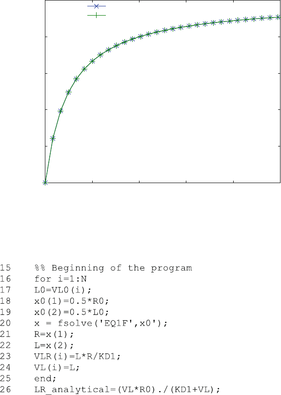
The main program basically contains a loop running from line 16 to line 25.
Loops are sets of commands which are executed over and over, until a condition is
fulfilled. The simplest condition is the number of repeats, which is N in line 16. The
command for i ¼ 1:N states that the index i begins at 1 and is increased by its
default value of 1 until i ¼ N. For each i, a different total ligand concentration L0
(line 17) is used from VL0, the vector of initial concentrations which had been
created in line 14. Lines 18 and 19 give the initial estimates and correspond to
(5.4) and (5.5). Line 20 calls the function fsolve. It requires the name of the
0
0.2
0.4
0.6
0.8
1
0 20 40 60 80 100
Concentration of [LR] (bound ligand)
Concentration of [L] (free li
g
and)
Equilibrium Binding curve (EQ1.m)
numeric
analytic
Fig. 5.1 Equilibrium-binding curve. Bound ligand versus free ligand is shown for 1 mM receptor
and an equilibrium dissociation constant of 10 mM. The values were computed with the program
EQ1.m as numeric approximations (x) and analytical solutions (+)
46 5 Equilibrium Binding
subroutine function 'EQ1F' where the equations are written. Note that the
name'EQ1F' is a string of characters as defined by single-quote ('). fsolve
also requires the vector x0 of initial estimates as an argument. The result in line 20
is the vector x. In lines 21 and 22, the elements of the vector x are translated into
the chemical notation as free receptor R and free ligand L, respectively. Line 23
defines VLR as the vector of complexes LR, employing (2.15). VL (line 24 ) simply
gives the vector of free ligand concentration L. The loop ends with an end
statement. Octave allows different end statements like endfor, endif,
endwhile and endfunction. Since MATLAB does not support this, we do
not make use of this Octave feature.
The loop creates the vectors VLR and VL of complex and free ligand, respec-
tively. Calculating the analytical solution in octave does not require a loop. Line 26
is octave code and looks identical to (3.1), but note that VL is a vector of
concentrations L. In line 26 all concentrations of bound ligand LR for all free
ligand concentrations L are calculated with one statement. The operator ./ (dot
followed by forward slash) in line 26 denot es an element-by-element division.
It corresponds to the element-by-element multiplication explained in Sect. 4.7.
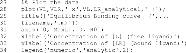
Once all relevant concentrations are calculated, they can be plotted with the plot
command given in line 28. The first argument in the plot function is the x-value, in
our case the free concentration vector VL and the second is the corresponding y-
value, the bound ligand vector VLR. The style (included in quotes) specifies line ()
and symbol (x). A second pair of x and y coordinates is supplied for the analytical
solution (LR_analytical). This is specified by another symbol (+). Lines 29 and 30
are remarkable for two reasons. First, the continuation marker (three dots) at the end
of a line indicates that the next line belongs to the same statement. In this case, lines
29 and 30 are pasted to a single title function. The second remarkable feature of
the
title function is the string which is given as an argument. Every string may be
regarded as a row vector of characters. In Octave, any row vector is defined by
its elements, separated by commas, in square brackets (Sect. 4.7). Therefore
['Equilibrium Binding curve (',filename,'.m)'] is a row vector of
the string 'Equilibrium Binding curve (', followed by the parameter string
filename (defined in line 8), followed by the string '.m)'.
The same procedure (row vector of strings) is used in the print and save
commands in lines 36, 37, 38 and 40. Unfortunately, Octave version 3.2.4 gives
a message implicit conversion from matrix to string whenever a
print command (line 36 and 37) is executed. Such a warning is not given when the
5.2 Equilibrium Binding to One Site (EQ1.m) 47
same program is run in MATLAB or older versions of Octave. Therefore, please
ignore the message implicit conversion from matrix to string
displayed in the Octave Terminal window of version 3.2.4.
The statement axis (line 31) requires a row vector of min and max values for
the x- and y-axes, respectively. The legend function (line 34) inserts a legend into
the plot, thus also relates to the plot function. The two strings correspond to the
two data pairs in the plot command of line 28. A third argument is a number (2, in
this case), which defines the quadrant in which the legend will appear.
The last lines of the program EQ1.m give examples for different output formats.
The print command in lines 36 and 37 is used to save the graphic output in two
graphic format s, namely .jpg (line 36 ) and .emf (line 37). The later format
(Microsoft-enhanced metafile) was used for all figures in this textbook. All
parameters can be saved with the save command in line 38. The data might be
retrieved at any time with a corresponding load command. Octave (not
MATLAB) stores the resulting data file EQ1_all.txt in an ASCII format
which can be accessed with any text editor. In both computer languages, the data
can be stored in ASCII format as a spreadsheet. This is done with the option
–ascii in line 40, but one can save only a single matrix with this comma nd.
Therefore, the matrix out was generated in line 39 as a row of the column vectors
of interest . Figure 5.1 is generated when EQ1 is typed in the Octave terminal or
MATLAB command window. As mentioned before, please ignore the two
messages implicit conversion from matrix to string. They appear
when Octave version 3.2.4 is used.
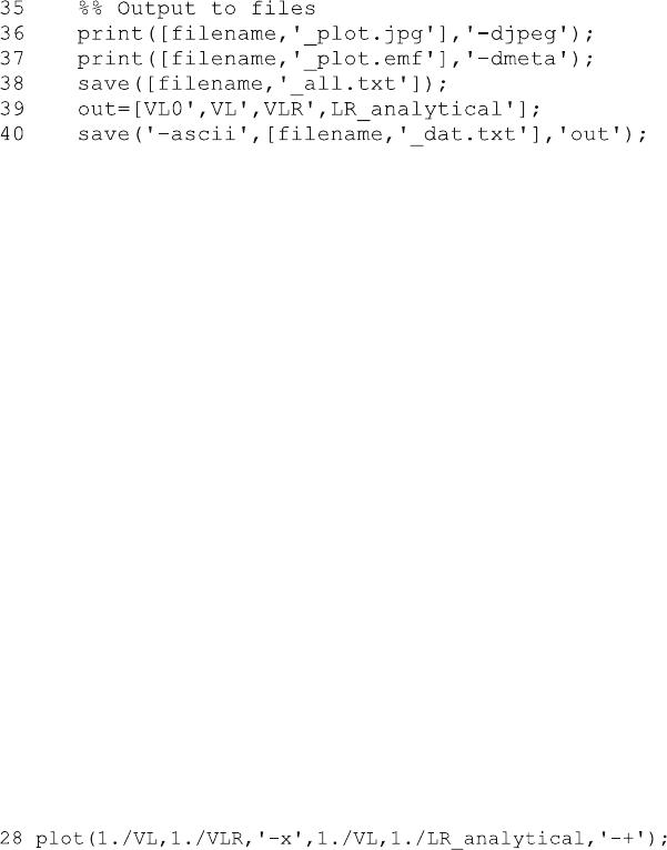
How to modify the sample program. All programs in this book are examples,
which can and should be modified so that they may be used as templates for other
problems. One possible modification of EQ1.m is shown in the program EQ2.m,
which calculated equilibrium binding to two sites. But there are numerous other
possibilities. Variables can be changed in lines 10–14. The plot may be modified
in line 28, and title, legends and labels in lines 29–34. Try it out! For example, if
you want to show your data as a double reciprocal plot, you simply modify line 28.
Note, however, that one cannot simply use a division for vectors. One has to use
element-by-element division (./):
If you only changed line 28 and run EQ1 in the octave terminal window, you
will get an empty plot, because you forgot to modify the axis. One may remove line
31 and the plot function will find its own default axes. Instead of removing a line, it
48 5 Equilibrium Binding
is easier to define it as a comment by adding the % (percent) character at the
beginning of line 31 to define it as a comment:
And ... voila, a double reciprocal plot appears when you enter EQ1 in the
terminal window. Of course, the axis labels are still wrong, but play with it. One
can easily modify everything.
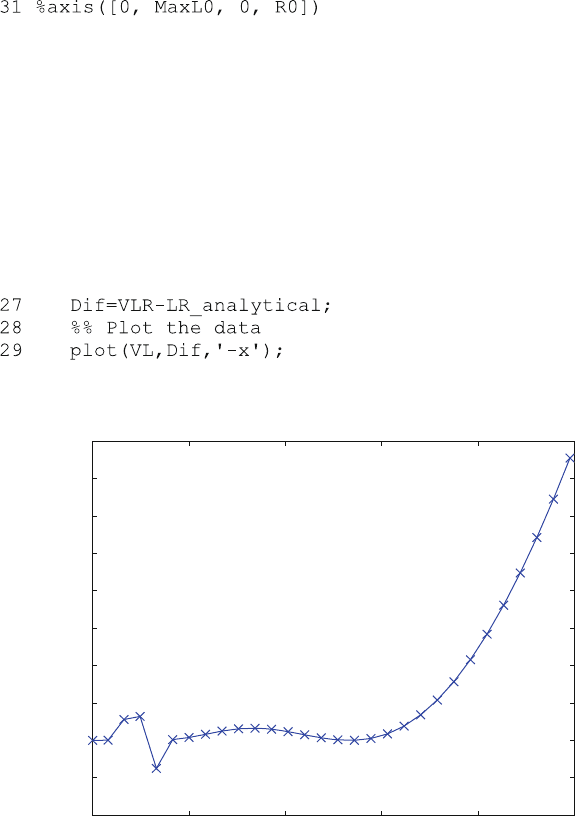
The program EQ1b.m is a modification of EQ1.m for the calculation of the
difference between numerical and anal ytical solutions. As discussed in Sect. 2.6,
numerical solutions are approximations, whereas analytical solutions always are
correct. For Octave 3.2.3 and its default parameters the differences between numer-
ical and analytical solutions of EQ1.m are shown in Fig. 5.2.
The differences were computed with EQ1b.m, a program which differs from
EQ1.m mainly in lines 27 and 29.
-2e-007
-1e-007
0
1e-007
2e-007
3e-007
4e-007
5e-007
6e-007
7e-007
8e-007
0 20 40 60 80 100
Concentration of [L] (free li
g
and)
Difference between numerical and analytical solutions (EQ1b.m)
Fig. 5.2 Differences between numerical and analytical solutions. Bound and free ligand
concentrations shown in Fig. 5.1 were calculated for 1 unit (mM) receptor and an equilibrium
dissociation constant of 10 units (mM). The differences of the numerical and analytical solution as
calculated with Octave version 3.2.3 are plotted versus the free ligand concentration. Note the
scale of the y-axis, which merely covers a total range of 10
6
units, corresponding to 1 pm, which
is not visible clearly in Fig. 5.1
5.2 Equilibrium Binding to One Site (EQ1.m) 49