Prinz H. Numerical Methods for the Life Scientist
Подождите немного. Документ загружается.

generally should not be used for data fitting because the experimental errors are not
proportional to the transformed data values. Fits to the original data are more
reliable. They require nonlinear fitting routines which are covered in Chap. 8.
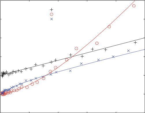
A simple binding curve (3.1) gives a straight line in a Scatchard plot ((+) in
Fig. 3.4). The interpolation to the x-axis gives the concentration of maximal bound
ligand. For one binding site on the receptor molecule, this is identical to the receptor
concentration R0. If there are two binding sites on the receptor, this value increases
by the factor 2. These sites may have different affinities for the same ligand. If one
binding site is characterized by an equilibrium dissociation constant of 10 mM,
and the other by 100 mM, the data show a marked curvature (x) in the Scatchard plot
(Fig. 3.4), whereas the same data almost appear linear in a double reciprocal
plot (Fig. 3.5). This is the reason why Scatchard plots have been used to distinguish
between cooperative (o) and noncooperative (x) binding. It should be mentioned
that a Scatchard Plot is the same as an Eadie-Hofstee plot when y- and x-axes are
exchanged.
The comparison of Figs. 3.4 and 3.5 shows that Scatchard plots are superior to
detect systematic deviations from simple binding equilibrium. Double reciprocal
plots always have a tendency to appear linear.
0
0.5
1
1.5
2
2.5
3
0 0.02 0.04 0.06 0.08 0.1
1 / bound ligand concentration
1 / free li
g
and concentration
Double reciprocal plot (ana4.m)
one binding site
cooperative binding
2 independent sites
Fig. 3.5 Double reciprocal plot (same data as shown in Fig. 3.4)R0¼ 1 mM. (+) Binding to one
site with K
D
¼ 10 mM. (o) Cooperative binding to two sites, K
D
1 ¼ 100 mM, K
D
2 ¼ 10 mM. (x)
Two independent binding sites with K
D
1 ¼ 10 mM, K
D
2 ¼ 100 mM. The theoretical curves
plotted are shown as solid lines. A random noise of 5% was assumed for both free and bound
ligand. Data points were calculated from logarithmic distributions of ligand concentrations
20 3 Classical Analytical Solutions
3.1.4 Lineweaver-Burk Plots
Enzymes are biopolymers which catalyze a biochemical reaction. In the simplest
case, an enzyme E binds a substrate S and forms the complex ES. The product P is
formed in the enzyme. Both the product formation and dissociation are first-order
processes. They may be combined to one first-order catalytic rate constant k
cat
so
that reaction scheme (3.4) may be used.
S þ E Ð
k
1
k
1
ES 0
k
cat
E þ P (3.4)
When the dissociation rate constant k
1
is much larger than k
cat
, only a fraction of
ES dissociates to E + P. When substrate is in large excess over E, only a tiny fraction
of S can bind and only a small part of this can be catalyzed to form P. In this case, the
initial equilibrium of S + E and ES is maintained for quite a while until a significant
amount of S has been used up by the catalysis. This initial part of such a reaction is
called “steady-state equilibrium” [6]. It can be computed just like any other equilib-
rium [7], with an equilibrium dissociation constant K
m
¼ (k
1
+k
cat
)/k
1
.K
m
is
called the Michaelis constant and steady-state enzyme kinetics of reaction scheme
(3.4) are referred to as “Michaelis-Menten kinetics” [5, 8–13].
The rate of product formation follows from first-order dissociation (2.6)
v ¼ d[P]/dt ¼ k
cat
[ES] (3.5)
The enzyme concentration E0 usually is more than a factor of hundred smaller
than the substrate concentration so that in the beginning of the reaction the free
ligand concentration does not differ significantly from the total ligand concentration
([L] ¼ L0). This gives a steady-state equilibrium, and the concentration of bound
substrate [ES] can be computed from (3.1). Substituting L with S0, R0 with E0, and
K
D
with K
m
leads to
v
0
¼ d[P]/dt ¼ k
cat
S0 E0/(S0 þ K
m
Þ (3.6)
The maximal velocity is
v
max
¼ k
cat
E0 (3.7)
and (3.6) becomes
v
0
¼ d[P]/dt ¼ v
max
S
0
=ðS
0
þ K
m
Þ (3.8)
Equation (3.8) is called Michaelis-Menten equation [5, 8–13]. It is basically the
same as (3.1), but it calculates the initial velocity of product formation (or substrate
depletion) rather than ligand binding. The Michaelis constant is equal to the
3.1 Analytical Solutions for Equilibrium Binding 21
equilibrium dissociat ion constant of substrate binding when k
cat
<< k
1
. Other
cases of steady-state approximations will not be discussed in this chapter, because
numerical methods allow correct calculations. The program enz2.m (Fig. 7.3)
calculates reaction scheme (3.4) without any restrictions imposed on the selection
of rate constants.
When the initial velocity is plotted versus the substrate concentration, the
resulting curve likewise is very similar to that shown in Figure 3.1.Itisan
equilibrium-binding curve attributed to the steady-state equilibrium of enzyme
kinetics. Sometimes this type of plot itself is referred to as “enzyme kinetics” or
“Michaelis-Menten kinetics.” Just as shown in (3.2) for direct binding curves,
taking the inverse of (3.8) will give
1=v
0
¼ðK
m
=v
max
Þ1=S
0
þ 1=v
max
(3.9)
Therefore, when 1/v0 is plotted versus 1/S0, the result will be a straight line with
a slope of K
m
/v
max
and an intersection 1/v
max
at the y-axis. The double reciprocal
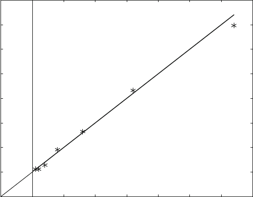
plot for enzyme kinetics is called Lineweaver-Burk plot [14] (Fig. 3.6).
0
10
20
30
40
50
60
70
80
-0.1 0 0.1 0.2 0.3 0.4 0.5 0.6 0.7
1 / [v0] (1/ initial velocity)
1 / S0
Lineweaver Burk Plot (ana5.m)
Fig. 3.6 Lineweaver-Burk plot. Double reciprocal plot of initial velocity and total substrate
concentration. Initial velocity is calculated from (3.8)withK
M
¼ 10 mM, E0 ¼ 10 nM, kcat ¼ 10 s
1
.
Intersection with the x-axis yields 1/K
M
, the intersection with the y-axis 1/v
max
. The theoretical
curve plotted is shown as a solid line. A random noise of 10% was assumed for the initial velocity.
Data points were calculated from a twofold dilution series of the substrate concentration beginning
with 100 mM
22 3 Classical Analytical Solutions
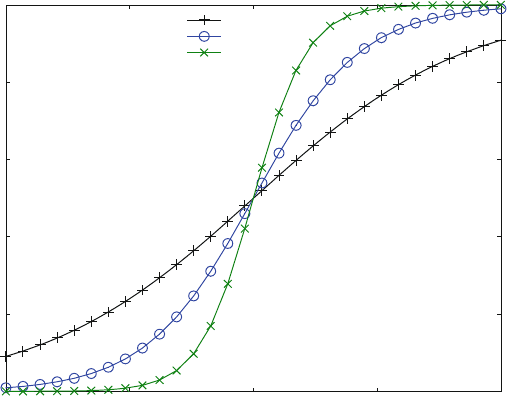
Figure 3.6 shows the calculation from substrate concentrations derived from a
twofold dilution series. Section 8.2 explains why such a series ensures a minimal
experimental error. Compari ng Figs. 3.6 and 3.3 shows that such a dilution series is
much more effective in covering a more significant data range. Only seven data
points were required for the calculation shown in Fig. 3.6.
3.1.5 Dose–Response Curves and Hill Coefficients
When drug binding to a receptor [1] leads to a physiological response, the intensity
of this response should follow the same curve as the binding curve (3.1). Such a
dose–response curve usually is plotted in a logarithmic scale, where a hyperbolic
function (Fig. 3.1) will look sigmoid ((+) in Fig. 3.7). In many cases, experiment al
dose–response curves do not follow (3.1). The maximal slope of the sigmoid
dose–response curve often is larger than that expected from binding to one site.
In this case, scheme (3.10), which had been used in 1910 for the binding of oxygen
to hemoglobin [15], often is used as an approximation.
nL þ R Ð L
n
R (3.10)
0
20
40
60
80
100
0 0.5 1 1.5 2
Response (% of maximal response)
log (ligand concentration)
Logistic dose-response curves (ana6.m)
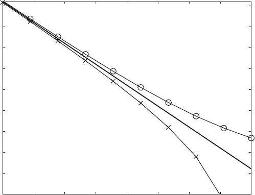
Binding curve, nH = 1
Logistic curve, nH = 2
Logistic curve, nH = 4
Fig. 3.7 Logistic dose–response curves. The binding curve (+) was calculated from (3.1), the
logistic curves from (3.12) with n ¼ 2 (o) and n ¼ 4 (x). K
D
or EC
50
was 10 mM
3.1 Analytical Solutions for Equilibrium Binding 23
Scheme (3.10) assumes simultaneous binding of n ligand molecules L to a
receptor R, without intermediates LR, L
1
R, L
2
R,...and the like. Such simultaneous
binding is unlikely in solution, but nevertheless (3.10) is commonly used for the
calculation of dose–response curves. It would lead to a binding function (3.11 )
½L
n
R] ¼ R0=ð1 þðK
D
/[L]Þ
n
Þ (3.11)
K
D
is the equilibrium dissociation constant for each step, n is called the Hill
coefficient, and is usually denoted as n
H
. Unlike n in (3.10) the Hill coefficient n in
(3.11) need not be an integer . Mathematically (2.11) is a logistic function, which
originally had been developed [16] for the description of population growth.
Logistic functions are easy to calculate and easy to fit. They are often applied to
dose–response curves as “4 parameter logistic equations” (3.12)
Response ¼ (Max Min)/(1 þ (EC
50
/x)
n
Þ (3.12)
With x as the drug concentration and the four parameters, Max ¼ maximal
amplitude, Min ¼ background, EC
50
¼ ligand concentration for the half-maximal
response and n ¼ n
H
¼ Hill coefficient, it has been pointed out that logistic
functions do not correspond to any realistic binding scheme unless the Hill coeffi-
cient is one [17, 18].
When logistic functions (3.12) are calculated for different Hill coefficients and
plotted versus the logarithm of the drug concentration, the result is a series of
symmetric sigmoid curves (Fig. 3.7). Such curves are very useful for fitting,
because the four parameters Max, Min, EC
50
and n
H
are usually not correlated
(Sect. 8.1). Modification of n
H
changes the shape of the curve. Its maximal slope
thus can be varied independent of the inflection point (EC
50
). Amplitude (Max) and
background (Min) can also be varied independently.
From the logistic dose–response curves in Fig. 3.7, only the binding curve (+)
with a Hill coefficient of 1 corresponds to a plausible reaction scheme (3.1 ).
Experimental dose–response curves were found to be unsym metrical when the
maximal slope was steeper than for the binding curve (+) shown in Fig. 3.7 [18].
For these types of experimental curves, there is no generally accepted explanatio n
[17, 18]. One new explanation for commonly observed steep dose–response curves
has been published [19]; another one is calculated from multiple allosteric
interactions (Fig. 5.12) and another one from irreversible reactions (Fig. 6.11).
3.2 Analytical Solutions for Binding Kinetics
The dissociation of ligand L from the receptor–ligand complex is a first-order
reaction as described in (2.6). Rearranging this equation gives
d[LR]/[LR] = k
1
dt (3.13)
24 3 Classical Analytical Solutions
This can be integrated from the initial concentration [LR]
0
(the equilibrium
concentration for t ¼ 0 at the beginning of the dissociation reaction) to the concen-
tration of [LR] at time t:
ð
½LR
½LR
0
d[LR=½LR¼k
1
ð
t
0
dt (3.14)
The analytical solution is:
ln [LR]ðÞ¼ln [LR]
0
ðÞk
1
t (3.15)
[LR] ¼ [LR]
0
e
k
1
t
(3.16)
Equation (3.15) states that the logari thm of [LR] should be a linear function of t.
Dissociation can easily be measured when a large excess of a competing ligand is
added to the complex LR. Since the forward reaction is blocked by the competitor,
only the dissociation reaction with the rate constant k
1
should be observed. This
type of experiment is extensively discussed and calculated in Sects. 6.4–6.6.
3.2.1 Exponential Decay
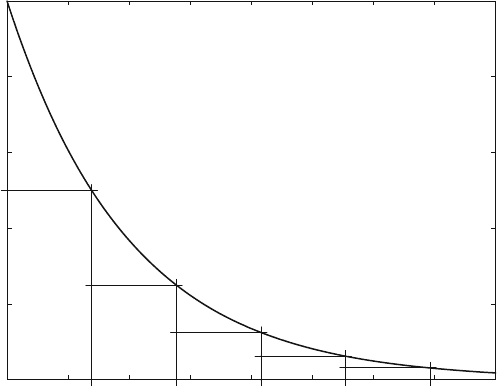
Equation (3.16) describes the exponential decrease of the complex [LR], and is
shown in Fig. 3.8. Equation (3.16) is based on (2.6) and theref ore can be applied
whenever the decay rate of a substance is proportional to its concentration. Such a
phenomenon is rather common in nature, with radioactive decay as the most
prominent example.
The time which is required for the dissociation of half of the molecules is called
“half life” and often is denoted with the Greek letter t (tau). From (3.15)or(3.16)
one can compute that t is equal to ln2/k. It is independent of the initial concentra-
tion and therefore would be the same for the decay from 100% to 50% or from 50%
to 25% and so forth. A dissociation reaction followed for more than five half-lives is
shown in Fig. 3.7 .
Measuring the half-life of a dissociation reaction is the simplest method for
obtaining the rate constant of this reaction: k ¼ ln2/t. It is also the simplest
method to ensure that a reaction truly is of the first order: Subsequent half-lives
must always give the same value, and one can begin to monitor a first-order reaction
at any time.
3.2 Analytical Solutions for Binding Kinetics 25
3.2.2 Half-Logarithmic Plots
Half-logarithmic plots of simple exponential decays should be linear, as they follow
(3.15). Experimental data often do not yield a linear half-logarithmic plot. In some
cases the dissociation reaction is more complex. In other cases, fluctuation of the
background signal may cause a deviation. Typically, one does not monitor absolute
concentrations, but will follow the reaction by a signal (fluorescence, NMR,
absorption,...) which is proportional to the concentration. Such a signal always
will have a background, and in order to take the logarithm of the signal in Fig. 3.8,
one has to take the logarithm of signal minus background. The background shown
in Fig. 3.8 would be the signal at “infinite” time, which translates to the signal after
at least ten half-lives. Fluctuations of the experimental points will lead to statistical
fluctuations, but fluctuations of the background will lead to systematic deviations as
shown in Fig. 3.9 .
Drifts in the background can also be caused by typical experimental artifacts,
such as bleaching, instability of a lamp, temperature increase and so forth. The half-
logarithmic plot of ln [LR] vs. time (3.15) should be linear, but background
variations may lead to distortions (Fig. 3.9). This may be one of the reasons why
half-logarithmic plots have disappeared with the introduction of personal
computers. Instead, one typically would fit (3.16) and add the background signal
as an additional parameter. It should be stated, however, that the initial part of a
0
20
40
60
80
100
0 0.5 1 1.5 2 2.5 3 3.5 4
Concentration of [LR] (bound ligand)
Time (seconds)
Exponential Decay (ana7.m)
Fig. 3.8 Exponential Decay. Equation (3.16) is calculated with a rate constant k
1
¼ 1s
1
, initial
concentration [LR]
0
¼ 100, t ¼ ln 2 s
26 3 Classical Analytical Solutions
complex reaction often is identical to one simple exponential curve and that
subsequent deviations may escape notice when background is used as a parameter
for curve fitting.
3.2.3 Initial Velocity of Association Kinetics
A reversible reaction may involve conformational changes and may be quite
complex, but the first part of an association reaction where a ligand L is added to
free receptor R (only one binding site) is simple at the time point t ¼ 0. When both
reaction partners meet for the first time, their initial free concentrations are equal to
the total concentrations:
v
0
¼ d[LR]/dtj
t¼0
¼ k
1
L0 R0 (3.17)
Experimentally, the initial velocity is easy to measure, since it is the tangent to a
kinetic experiment at zero time. At zero time, there is no bound ligand formed so
that all back reactions can be ignored. When the concentration change of LR can be
quantified and when the initial concentrations L0 and R0 are known, the rate
constant k
1
of the initial part of the association reaction can be determined without
curve fitting.
0
0.5
1
1.5
2
2.5
3
3.5
4
4.5
0 0.5 1 1.5 2 2.5 3 3.5 4
ln (Concentration of [LR])
Time (seconds)
Half-logarithmic plot (ana8.m)
Fig. 3.9 Half-logarithmic plot of the reaction in Fig. 3.8. Equation (3.16) with k
1
¼ 1s
1
,
[LR]
0
¼ 100 is calculated. () Logarithm of [LR]. (o) 2% background was added before the
logarithm was taken, (x) 2% background
3.2 Analytical Solutions for Binding Kinetics 27
3.2.4 Pseudo First-Order Kinetics
The rate of a second-order reaction (2.1) is proportional to the concentration of both
reactants (2.2). If one of these concentrations is kept constant, the rate is only
proportional to the other. This results in a “pseudo” first-order reaction. If L0
is more than a factor of ten larger than R0, the free ligand concentration L0 of a
reversible reaction (2.9) does not change significantly upon binding and therefore can
be regarded as constant so that the differential equation for [LR] can be simplified:
dLR½/dt ¼ k
1
L0 R½k
1
LR½
dLR½/dt ¼ k
1
L0 R0 LR½ðÞk
1
LR½
dLR½/dt ¼ k
1
L0 þ k
1
ðÞLR½þk
1
L0 R0
(3.18)
This is, apart from the constant k
1
· L0 · R0, the same as (3.13). Integration
leads to
ln [LR]ðÞ¼const ðk
1
L0 þ k
1
Þt (3.19)
This is the same as an exponential decay (3.15) and (3.16) with an observed rate
constant k
k ¼ k
1
L0 þ k
1
(3.20)
If one measures binding kinetics at different concentrations of L0 (the ligand in
excess), one can obtain a series of pseudo first-order rate constants k. If one plots
these constants versus the concentrations of excess ligand, the result is a straight
line with a slope of k
1
and an intersection with the y-axis of k
1
. It should be noted
that (3.20) is independent of the direction of the reaction. If the reaction is started
from a complex LR, and if this complex is diluted by a large factor, then the
observed dissociation also would follow first-order kinetics with the pseudo first-
order rate constant k from (3.19).
3.2.5 Multiple Exponential Fits
In many cases, binding kinetics is complex and cannot be fitted to simple
exponentials. Sometimes the following sum is used to fit the experimental data:
[LR] ¼ A1 e
k1t
+A2 e
k2t
+A3 e
k3t
þ ... (3.21)
This is a sum of exponential functions with amplitudes A1, A2, A3,... and rate
constants k1, k2, k3,.... Almost all curves can be fitted with such a sum of
exponential curves. The resulting amplitudes and rate constants are not very
28 3 Classical Analytical Solutions
meaningful since generally there is no plausible reaction scheme which would lead
to (3.21). Sometimes (3.21) is used simply as a way to describe the data. This is
correct, as long as the whole ensembl e of parameters (rate constants and
amplitudes) is reported. One should note that the parameters of (3.21) generally
are correlated so that individual rate constants cannot be extracted from a fit with
(3.21), unless they are significantly more than one order of magnitude apart.
Correlation is discussed in Sect. 8.1. Note that k1, k2, k3,... of a multi exponential
fit in a kinetic experiment are real numbers, and that (3.21) does not describe an
exponential Fourier series.
If an association reaction under pseudo first-order conditions does not give a single
exponential, then the reaction is more complex. The kinetics of such a model can only
be calculated from sets of differential equations and require numerical methods.
References
1. Langley JN (1905) On the reaction of cells and of nerve-endings to certain poisons, chiefly as
regards the reaction of striated muscle to nicotine and to curare. J Physiol 33:374–413
2. http://de.wikipedia.org/wiki/Scatchard-Diagramm
3. http://en.dogeno.us/2004/03/scatchard-plot/
4. Voet DJ, Voet JG (1995) Biochemistry. John Wiley & Sons, New York
5. Gutfreund H (1995) Kinetics for the life sciences. Receptors, transmitters and catalysts.
Cambridge University press, Cambridge
6. Segel LA, Slemrod M (1989) The quasi-steady-state assumption: a case study in perturbation.
SIAM Rev 31:446–477. doi:10.1137/1031091
7. Michaelis L, Menten ML (1913) Die Kinetik der Invertin-Wirkung. Biochem Z 49:333–369
8. Segel IH (1993) Enzyme kinetics: behavior and analysis of rapid equilibrium and steady-state
enzyme systems. Wiley Classical Library, New York
9. Copeland RA (2005) Evaluation of enzyme inhibitors in drug discovery: a guide for medicinal
chemists and pharmacologists. Wiley-VCH, Weinheim
10. Copeland RA (2000) Enzymes: a practical introduction to structure, mechanism, and data
analysis. Wiley, New York
11. Purich DL (2010) Enzyme kinetics: catalysis & control: a reference of theory and best-
practice methods. Elsevier, London
12. Cook PF, Cleland WW (2007) Enzyme kinetics and mechanism. Garland Science, New York
13. Leskovac V (2003) Comprehensive enzyme kinetics, Kindle Edition. Amazon
14. Lineweaver H, Burk D (1934) The determination of enzyme dissociation constants. J Am
Chem Soc 56:658–666
15. Hill AV (1910) The possible effects of the aggregation of the molecules of haemoglobin on its
dissociation curves. J Physiol (Lond) 40:iv–vii
16. Verhulst PF (1845) Recherches mathe
´
matiques sur la loi d’accroissement de la population.
Nouv me
´
m de l’Academie Royale des Sci et Belles-Lettres de Bruxelles 18:1–41
17. Weiss JN (1997) The Hill equation revisited: uses and misuses. FASEB J 11:835–841
18. Prinz H (2010) Hill coefficients, dose-response curves and allosteric mechanisms. J Chem
Biol 3:37–44
19. Prinz H, Sch
€
onichen A (2008) Transient binding patches: a plausible concept for drug binding.
J Chem Biol 1:95–104
References 29