Power electronic handbook

Подождите немного. Документ загружается.

30 M. G. Simoes

Saturation

region

Constant-current

(active) region

= i

Increasing

base current

, sat

(a) (b)

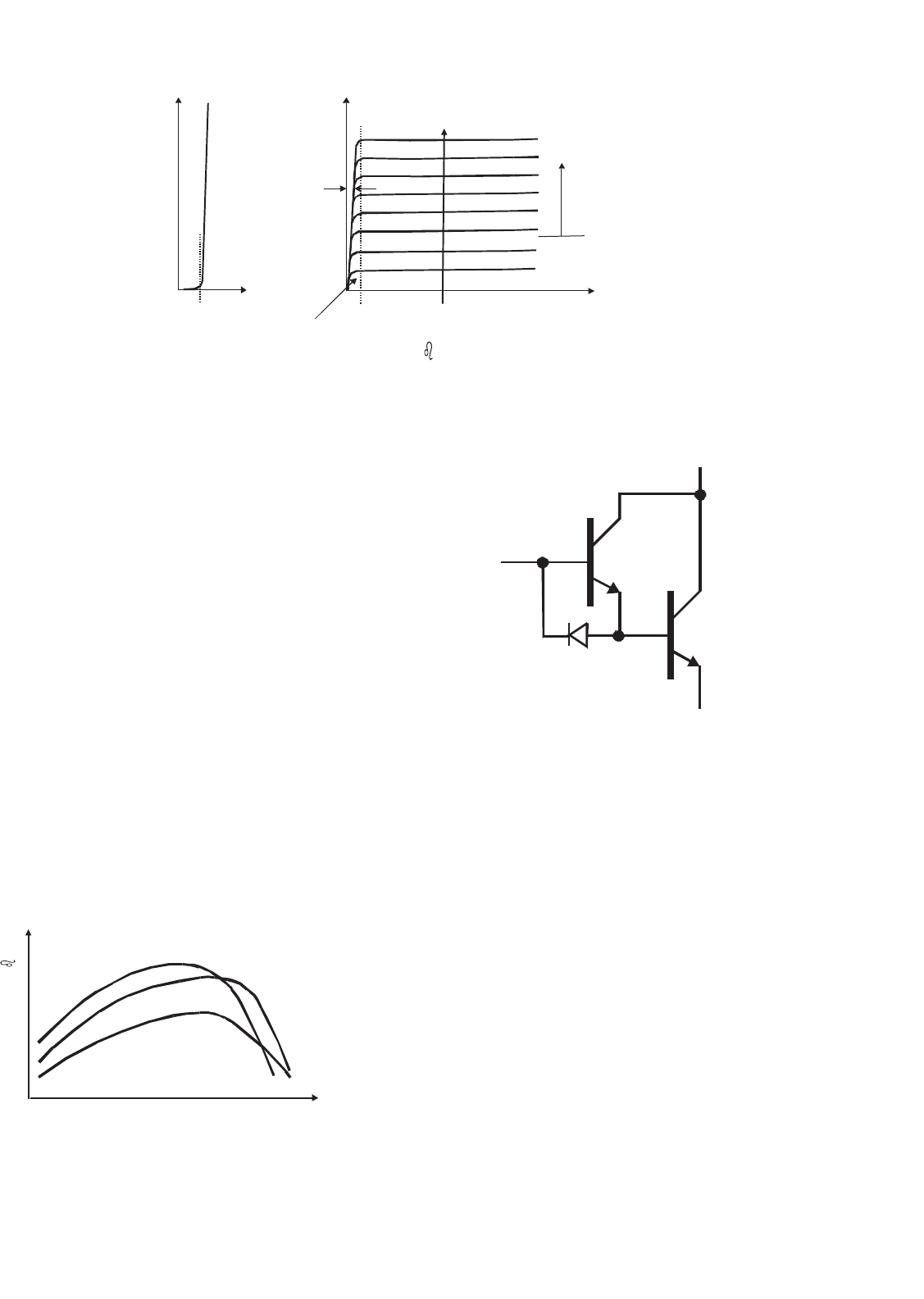
FIGURE 3.5 Family of current–voltage characteristic curves: (a) base–emitter input port and (b) collector–emitter output port.

a temperature rise and are related to the thermal resistance.

A family of voltage–current characteristic curves is shown in

Fig. 3.5. Figure 3.5a shows the base current i

plotted as a

function of the base–emitter voltage V

and Fig. 3.5b depicts

the collector current i

as a function of the collector–emitter

voltage V

with i

as the controlling variable.

Figure 3.5 shows several curves distinguished each other by

the value of the base current. The active region is deﬁned

where ﬂat, horizontal portions of voltage–current curves show

“constant” i

current, because the collector current does not

change signiﬁcantly with V

for a given i

. Those portions

are used only for small signal transistor operating as linear

ampliﬁers. Switching power electronics systems on the other

hand require transistors to operate in either the saturation

region where V

is small or in the cut off region where the

current is zero and the voltage is uphold by the device. A small

base current drives the ﬂow of a much larger current between

collector and emitter, such gain called beta (Eq. (3.4)) depends

upon temperature, V

and i

. Figure 3.6 shows current gain

increase with increased collector voltage; gain falls off at both

high and low current levels.

Current Gain ( )

log(i

)

= 2 V (25 °C)

= 400 V (25 °C)

= 2 V (125 °C)

FIGURE 3.6 Current gain depends on temperature, V

and i

FIGURE 3.7 Darlington connected BJTs.

High voltage BJTs typically have low current gain, and hence

Darlington connected devices, as indicated in Fig. 3.7 are com-

monly used. Considering gains β

and β

for each one of those

transistors, the Darlington connection will have an increased

gain of β

+β

, diode D

speedsup the turn-off pro-

cess, by allowing the base driver to remove the stored charge

on the transistor bases.

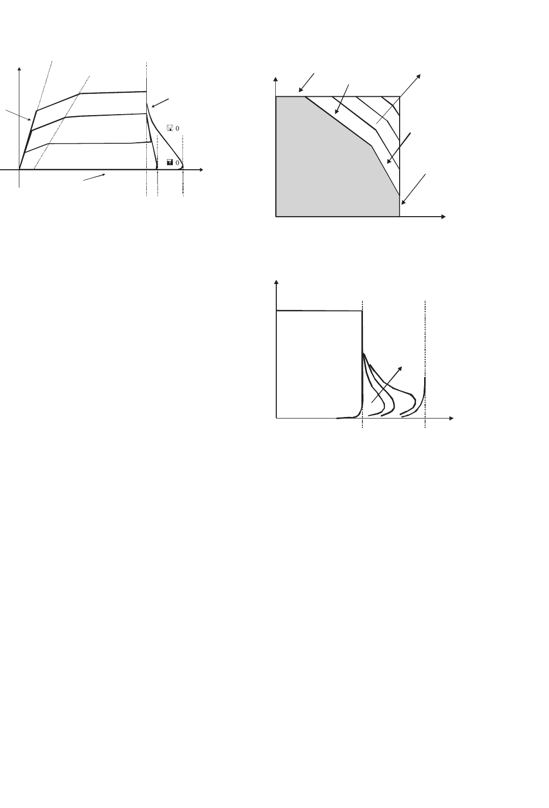
Vertical structure power transistors have an additional

region of operation called quasi-saturation, indicated in the

characteristics curve of Fig. 3.8. Such feature is a conse-

quence of the lightly doped collector drift region where the

collector–base junction supports a low reverse bias. If the tran-

sistor enters in the hard-saturation region the on-state power

dissipation is minimized, but has to be traded off with the fact

that in quasi-saturation the stored charges are smaller. At high

collector currents beta gain decreases with increased tem-

perature and with quasi-saturation operation such negative

feedback allows careful device paralleling. Two mechanisms

on microelectronic level determine the fall off in beta, namely

3 Power Bipolar Transistors 31

hard

saturation

quasi-saturation

constant-current

cut-off

SUS

CBO

breakdown

CEO

FIGURE 3.8 Voltage–current characteristics for a vertical power tran-

sistor.

conductivity modulation and emitter crowding. One can note

that there is a region called primary breakdown due to conven-

tional avalanche of the C–B junction and the attendant large

ﬂow of current. The BV

SUS

is the limit for primary break-

down, it is the maximum collector–emitter voltage that can be

sustained across the transistor when it is carrying high col-

lector current. The BV

SUS

is lower than BV

CEO

or BV

CBO

which measure the transistor’s voltage standoff capability when

the base current is zero or negative. The bipolar transistor

have another potential failure mode called second breakdown,

which shows as a precipitous drop in the collector–emitter

voltage at large currents. Because the power dissipation is not

uniformly spread over the device but it is rather concentrated

on regions make the local gradient of temperature can rise

very quickly. Such thermal runaway brings hot spots which

can eventually melt and recrystallize the silicon resulting in the

device destruction. The key to avoid second breakdown is to

(1) keep power dissipation under control, (2) use a controlled

rate of change of base current during turn-off, (3) use of pro-

tective snubbers circuitry, and (4) positioning the switching

trajectory within the safe operating area (SOA) boundaries.

In order to describe the maximum values of current and

voltage, to which the BJT should be subjected two diagrams,

are used: the forward-bias safe operating area (FBSOA) given

in Fig. 3.9 and the reverse-bias safe operating area (RBSOA)

shown in Fig. 3.10. In the FBSOA the current I

is the max-

imum current of the device, there is a boundary deﬁning the

maximum thermal dissipation and a margin deﬁning the sec-

ond breakdown limitation. Those regions are expanded for

switching mode operation. Inductive load generates a higher

peak energy at turn-off than its resistive counterpart. It is then

possible to have a secondary breakdown failure if RBSOA is

exceeded. A reverse base current helps the cut off character-

istics expanding RBSOA. The RBSOA curve shows that for

voltages below V

CEO

the safe area is independent of reverse

bias voltage V

and is only limited by the device collector

current, whereas above V

CEO

the collector current must be

CE0

Secondary

breakdown

limit

CEO

)

limit

tot

limit

Pulsed-SOA

FIGURE 3.9 Forward-bias safe operating area (FBSOA).

CE0

CB0

Reverse-bias

voltage V

FIGURE 3.10 Reverse-bias safe operating area (RBSOA).

under control depending upon the applied reverse-bias volt-

age, in addition temperature effects derates the SOA. Ability

for the transistor to switch high currents reliably is thus deter-

mined by its peak power handling capabilities. This ability is

dependent upon the transistor’s current and thermal density

throughout the active region. In order to optimize the SOA

capability, the current density and thermal density must be

low. In general, it is the hot spots occurring at the weakest

area of the transistor that will cause a device to fail due to

second breakdown phenomena. Although a wide base width

will limit the current density across the base region, good heat

sinking directly under the collector will enable the transistor

to withstand high peak power. When the power and heat are

spread over a large silicon area, all of these destructive tenden-

cies are held to a minimum, and the transistor will have the

highest SOA capability.

When the transistor is on, one can ignore the base cur-

rent losses and calculate the power dissipation on the on state

(conduction losses) by Eq. (3.5). Hard saturation minimizes

32 M. G. Simoes

collector–emitter voltage, decreasing on-state losses.

= I

CE(sat)

(3.5)

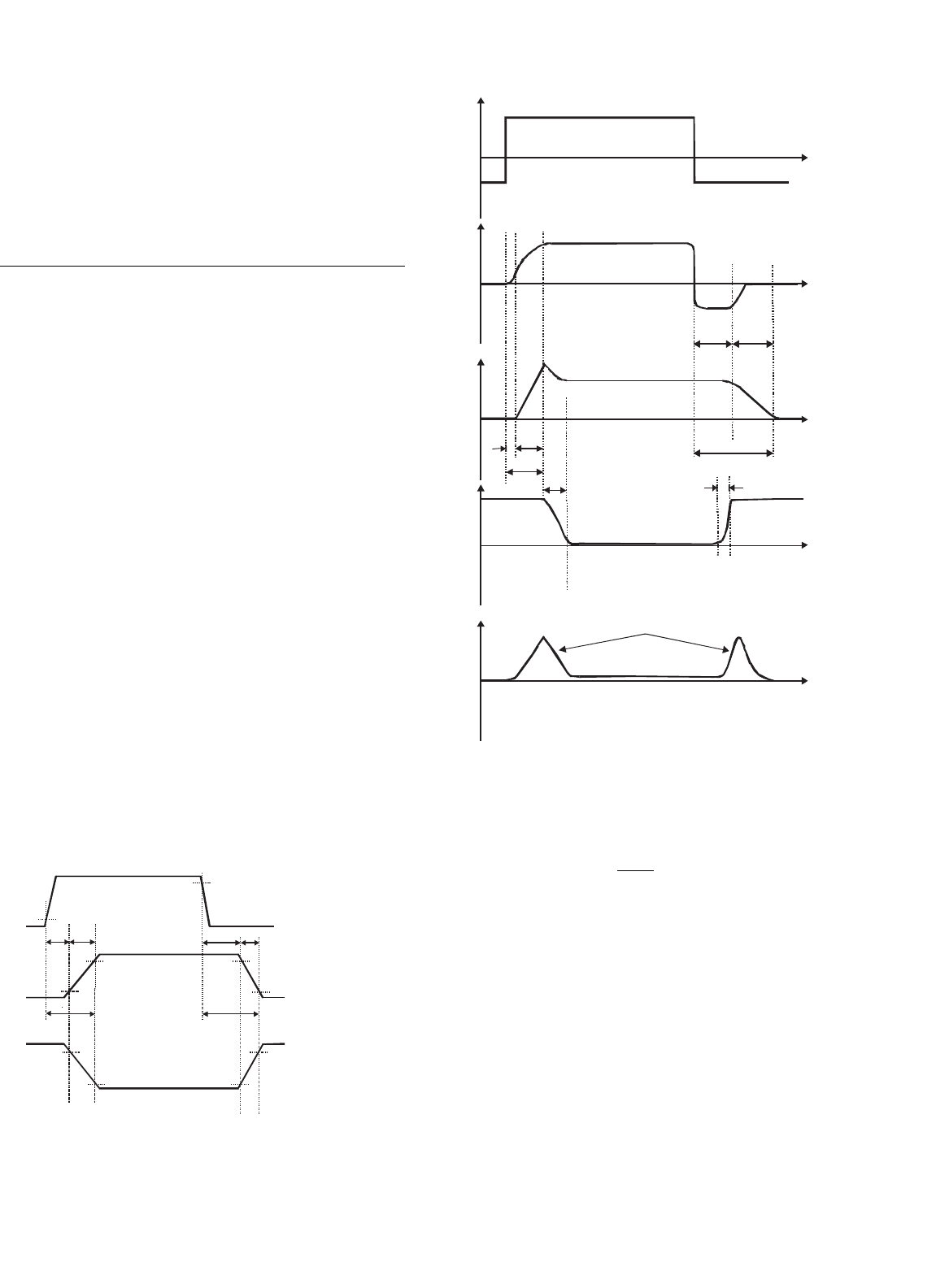
3.4 Dynamic Switching Characteristics

Switching characteristics are important to deﬁne the device

velocity in changing from conduction (on) to blocking (off)

states. Such transition velocity is of paramount importance

also because most of the losses are due to high-frequency

switching. Figure 3.11 shows typical waveforms for a resistive

load. Index “r” refers to the rising time (from 10 to 90% of

maximum value), for example t

is the current rise time which

depends upon the base current. The falling time is indexed by

“f”; the parameter t

ﬁ

is the current falling time, i.e. when the

transistor is blocking such time corresponds to crossing from

the saturation to the cut off state. In order to improve t

ﬁ

the

base current for blocking must be negative and the device must

be kept in quasi-saturation to minimize the stored charges.

The delay time is denoted by t

, corresponding to the time

to discharge the capacitance of base–emitter junction, which

can be reduced with a larger current base with high slope.

Storage time (t

) is a very important parameter for BJT tran-

sistor, it is the required time to neutralize the carriers stored

in the collector and base. Storage time and switching losses are

key points to deal extensively with bipolar power transistors.

Switching losses occur at both turn-on and turn-off and for

high frequency operation the rising and falling times for volt-

age and current transitions play important role as indicated by

Fig. 3.12.

A typical inductive load transition is indicated in Fig. 3.13.

The ﬁgure indicates a turn-off transition. Current and voltage

are interchanged at turn-on and an approximation based upon

on straight line switching intervals (resistive load) gives the

90%

10%

CE, SAT

Base current

Collector current

Voltage V

10%

90%

off

FIGURE 3.11 Resistive load dynamic response.

Switching losses

Conduction losses

CE, SAT

Collector current

Base voltage

Base current

Voltage V

Power

off

FIGURE 3.12 Inductive load switching characteristics.

switching losses by Eq. (3.6).

τf

(3.6)

where τ is the period of the switching interval, and V

and

are the maximum voltage and current levels as shown in

Fig. 3.10.

Most advantageous operation is achieved when fast tran-

sitions are optimized. Such requirement minimizes switching

losses. Therefore, a good bipolar drive circuit highly inﬂu-

ences the transistor performance. A base drive circuit should

provide a high forward base drive current (I

) as indicated in

Fig. 3.14 to ensure the power semiconductor turn-on quickly.

Base drive current should keep the BJT fully saturated to mini-

mize forward conduction losses, but a level I

would maintain

the transistor in quasi-saturation avoiding excess of charges

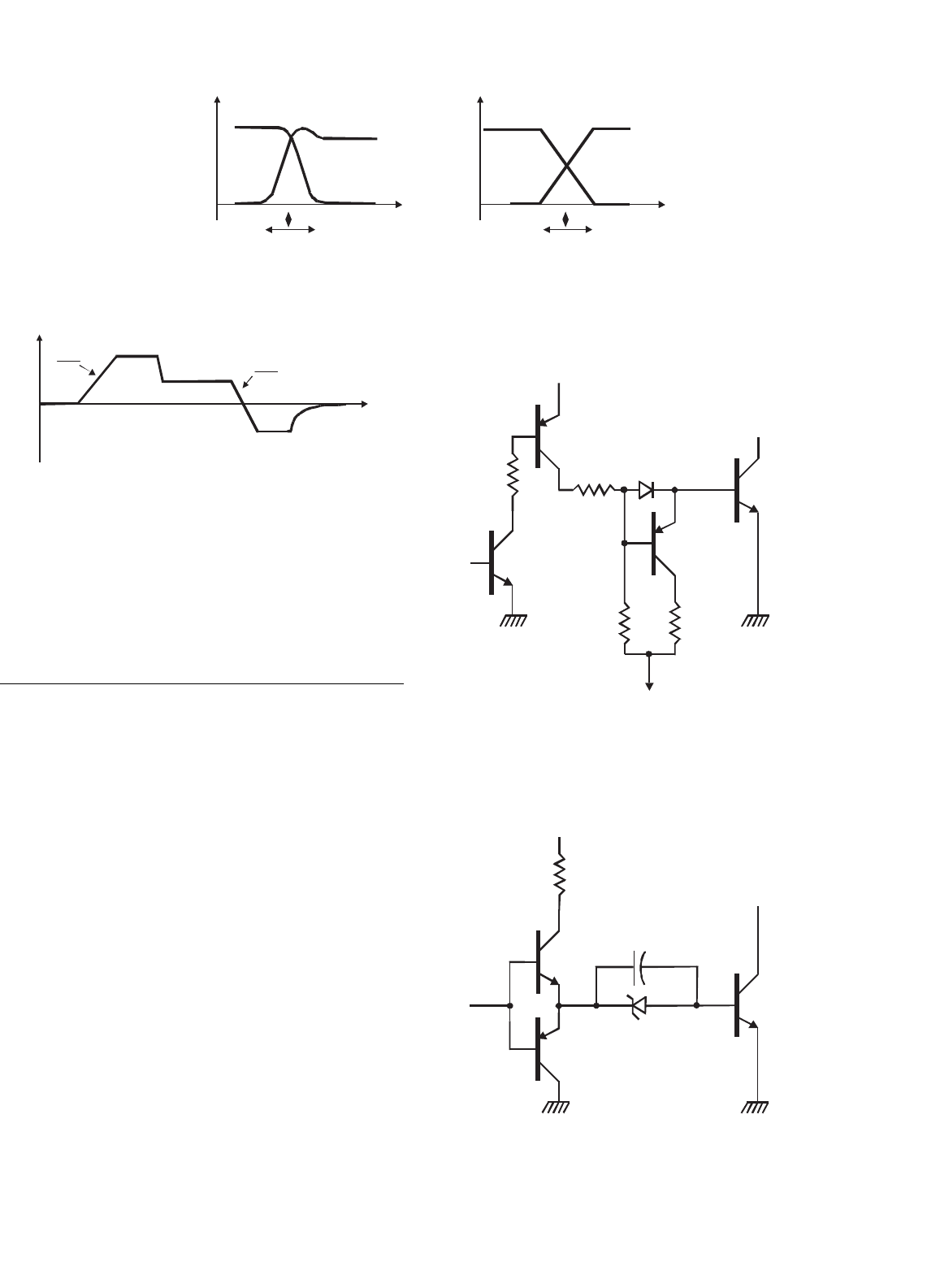
3 Power Bipolar Transistors 33

Voltage,

Current

Voltage,

Current

(a) (b)

FIGURE 3.13 Turn-off voltage and current switching transition: (a) inductive load and (b) resistive load.

FIGURE 3.14 Recommended base current for BJT driving.

in base. Controllable slope and reverse current I

sweeps out

stored charges in the transistor base, speeding up the device

turn-off.

3.5 Transistor Base Drive Applications

A plethora of circuits have been suggested to successfully com-

mand transistors for operating in power electronics switching

systems. Such base drive circuits try to satisfy the following

requirements: supply the right collector current, adapt the

base current to the collector current, and extract a reverse cur-

rent from base to speed up the device blocking. A good base

driver reduces the commutation times and total losses, increas-

ing efﬁciency and operating frequency. Depending upon the

grounding requirements between the control and the power

circuits, the base drive might be isolated or non-isolated types.

Fig. 3.15 shows a non-isolated circuit. When T

is switched

on T

is driven and diode D

is forward-biased providing a

reverse-bias keeping T

off. The base current I

is positive and

saturates the power transistor T

. When T

is switched off,

switches on due to the negative path provided by R

, and

–V

, providing a negative current for switching off the power

transistor T

When a negative power supply is not provided for the base

drive, a simple circuit like Fig. 3.16 can be used in low power

applications (step per motors, small dc–dc converters, relays,

pulsed circuits). When the input signal is high, T

switches

on and a positive current goes to T

keeping the capacitor

charged with the zener voltage, when the input signal goes low

–V

FIGURE 3.15 Non-isolated base driver.

FIGURE 3.16 Base command without negative power supply.

34 M. G. Simoes

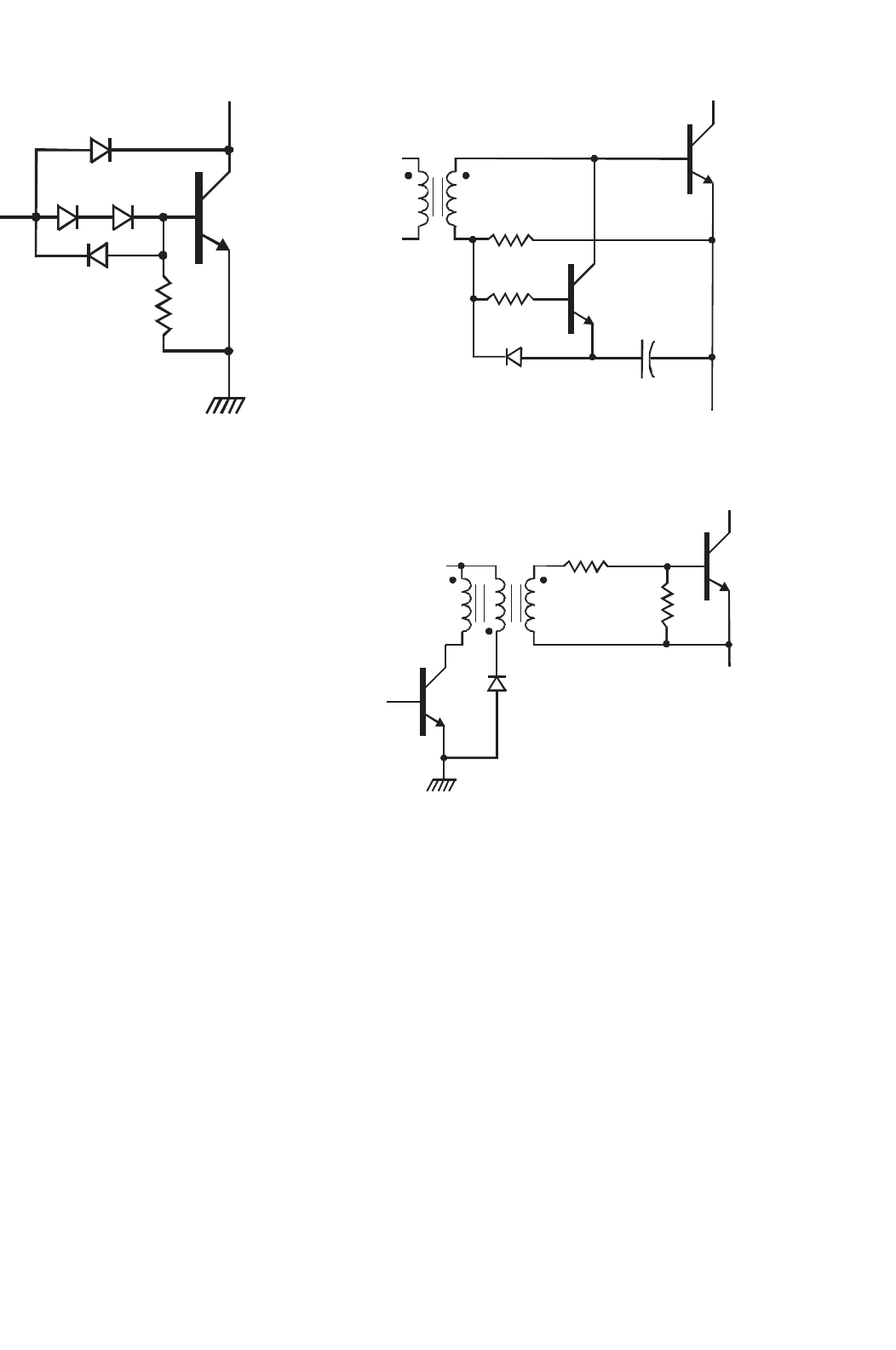
FIGURE 3.17 Antisaturation diodes (Baker’s clamp) improve power

transistor storage time.

provides a path for the discharge of the capacitor, imposing

a pulsed negative current from the base–emitter junction of T

A combination of large reverse base drive and antisaturation

techniques may be used to reduce storage time to almost zero.

A circuit called Baker’s clamp may be employed as illustrated

in Fig. 3.17. When the transistor is on, its base is two diode

drops below the input. Assuming that diodes D

and D

have a

forward-bias voltage of about 0.7 V, then the base will be 1.4 V

below the input terminal. Due to diode D

the collector is one

diode drop, or 0.7 V below the input. Therefore, the collector

will always be more positive than the base by 0.7 V, staying

out of saturation, and because collector voltage increases, the

gain β also increases a little bit. Diode D

provides a negative

path for the reverse base current. The input base current can

be supplied by a driver circuit similar to the one discussed in

Fig. 3.15.

Several situations require ground isolation, off-line oper-

ation, ﬂoating transistor topology, in addition safety needs

may call for an isolated base drive circuit. Numerous cir-

cuits have been demonstrated in switching power supplies

isolated topologies, usually integrating base drive requirements

with their power transformers. Isolated base drive circuits may

provide either constant current or proportional current exci-

tation. A very popular base drive circuit for ﬂoating switching

transistor is shown in Fig. 3.18. When a positive voltage is

impressed on the secondary winding (V

)ofT

a positive

current ﬂows into the base of the power transistor T

which

switches on (resistor R

limits the base current). The capac-

itor C

is charged by (V

–V

) and T

is kept blocked

because the diode D

reverse biases T

base–emitter. When V

is zipped off, the capacitor voltage V

brings the emitter of T

to a negative potential with respect to its base. Therefore, T

is excited so as to switch on and start pulling a reverse cur-

rent from T

base. Another very effective circuit is shown in

FIGURE 3.18 Isolated base drive circuit.

FIGURE 3.19 Transformer coupled base drive with tertiary winding

transformer.

Fig. 3.19 with a minimum number of components. The base

transformer has a tertiary winding which uses the energy stored

in the transformer to generate the reverse base current during

the turn-off command. Other conﬁgurations are also possible

by adding to the isolated circuits the Baker clamp diodes, or

zener diodes with paralleled capacitors.

Sophisticated isolated base drive circuits can be used to pro-

vide proportional base drive currents where it is possible to

control the value of β, keeping it constant for all collector cur-

rents leading to shorter storage time. Figure 3.20 shows one of

the possible ways to realize a proportional base drive circuit.

When transistor T

turns on, the transformer T

is in nega-

tive saturation and the power transistor T

is off. During the

time that T

is on, a current ﬂows through winding N

, lim-

ited by resistor R

, storing energy in the transformer, holding

3 Power Bipolar Transistors 35

FIGURE 3.20 Proportional base drive circuit.

it into saturation. When the transistor T

turns off, the energy

stored in N

is transferred to winding N

, pulling the core

from negative to positive saturation. The windings N

and N

will withstand as a current source, the transistor T

will stay

on and the gain β will be imposed by the turns ratio given by

Eq. (3.7).

β =

(3.7)

In order to use the proportional drive given in Fig. 3.20 careful

design of the transformer must be done, so as to have ﬂux

balanced which will keep core under saturation. The transistor

gain must be somewhat higher than the value imposed by

the transformer turns ratio, which requires cautious device

matching.

The most critical portion of the switching cycle occurs

during transistor turn-off, since normally reverse base cur-

rent is made very large in order to minimize storage time,

such conditions may avalanche the base–emitter junction lead-

ing to destruction. There are two options to prevent this

from happening: turning off the transistor at low values of

collector–emitter voltage (which is not practical in most of the

applications) or reducing collector current with rising collec-

tor voltage, implemented by RC protective networks called

snubbers. Therefore, an RC snubber network can be used

to divert the collector current during the turn-off improv-

ing the RBSOA in addition the snubber circuit dissipates a fair

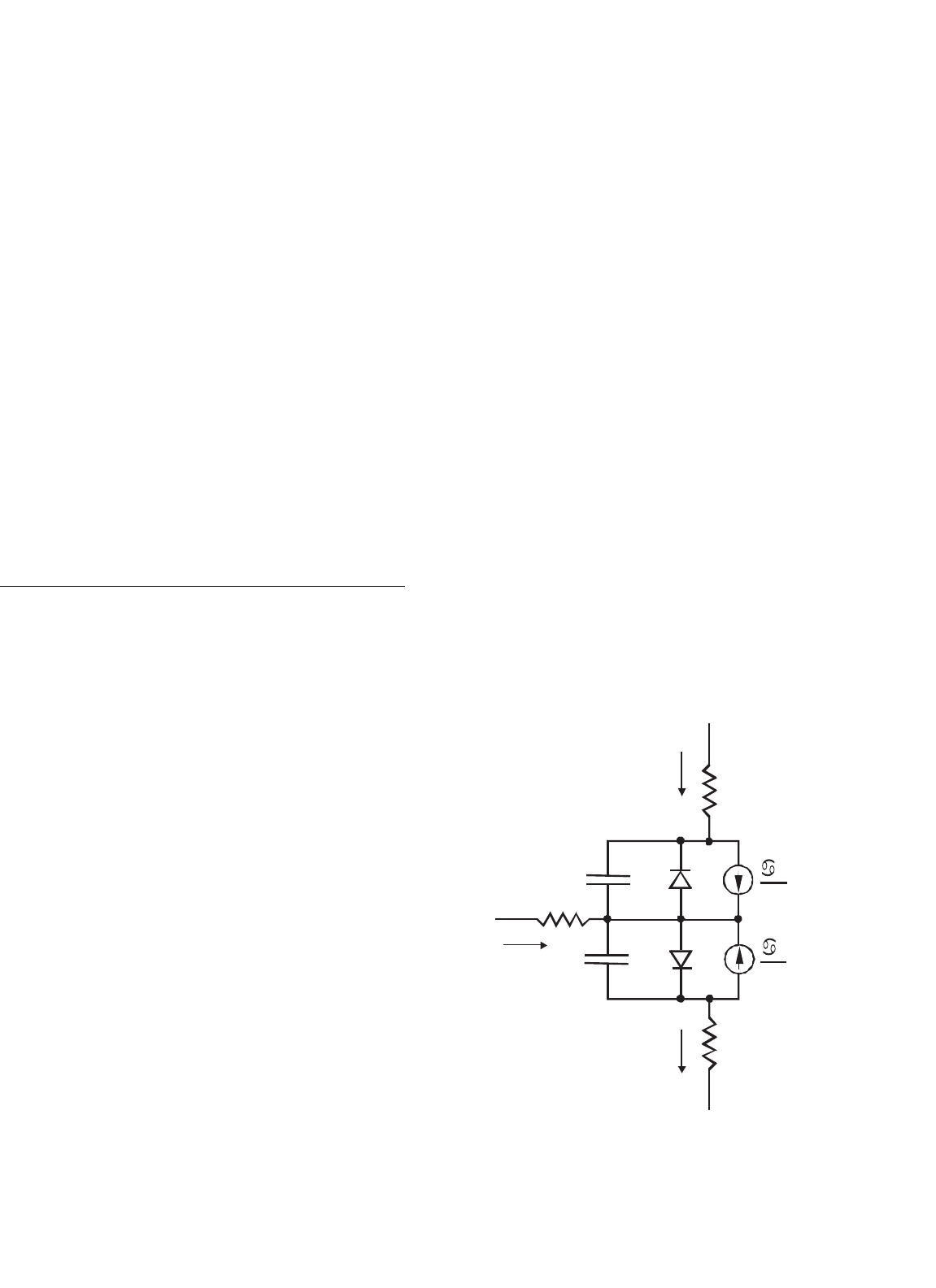
amount of switching power relieving the transistor. Figure 3.21

shows a turn-off snubber network; when the power tran-

sistor is off, the capacitor C is charged through diode D

Such collector current ﬂows temporarily into the capacitor as

the collector-voltage rises; as the power transistor turns on,

FIGURE 3.21 Turn-off snubber network.

the capacitor discharges through the resistor R back into the

transistor.

It is not possible to fully develop all the aspects regard-

ing simulation of BJT circuits. Before giving an example some

comments are necessary regarding modeling and simulation

of BJT circuits. There are a variety of commercial circuit sim-

ulation programs available on the market, extending from a

set of functional elements (passive components, voltage con-

trolled current sources, semiconductors) which can be used

to model devices, to other programs with the possibility of

36 M. G. Simoes

implementation of algorithm relationships. Those streams are

called subcircuit (building auxiliary circuits around a SPICE

primitive) and mathematical (deriving models from internal

device physics) methods. Simulators can solve circuit equa-

tions exactly, given models for the non-linear transistors, and

predict the analog behavior of the node voltages and currents

in continuous time. They are costly in computer time and such

programs have not been written to usually serve the needs of

designing power electronic circuits, rather for designing low-

power and low-voltage electronic circuits. Therefore, one has

to decide which approach should be taken for incorporating

BJT power transistor modeling, and a trade-off between accu-

racy and simplicity must be considered. If precise transistor

modeling are required subcircuit oriented programs should

be used. On the other hand, when simulation of complex

power electronic system structures, or novel power electronic

topologies are devised, the switch modeling should be rather

simple, by taking in consideration fundamental switching

operations, and a mathematical oriented simulation program

should be used.

3.6 SPICE Simulation of Bipolar

Junction Transistors

SPICE is a general-purpose circuit program that can be applied

to simulate electronic and electrical circuits and predict the

circuit behavior. SPICE was originally developed at the Elec-

tronics Research Laboratory of the University of California,

Berkeley (1975), the name stands for: Simulation Program

for Integrated Circuits Emphasis. A circuit must be speciﬁed

in terms of element names, element values, nodes, variable

parameters, and sources. SPICE can do several types of circuit

analyses:

•

Non-linear dc analysis, calculating the dc transference.

• Non-linear transient analysis: calculates signals as a

function of time.

•

Linear ac analysis: computes a bode plot of output as a

function of frequency.

• Noise analysis.

•

Sensitivity analysis.

• Distortion analysis.

• Fourier analysis.

•

Monte-Carlo analysis.

In addition, PSpice has analog and digital libraries of stan-

dard components such as operational ampliﬁers, digital gates,

ﬂip-ﬂops. This makes it a useful tool for a wide range of analog

and digital applications. An input ﬁle, called source ﬁle, con-

sists of three parts: (1) data statements, with description of the

components and the interconnections, (2) control statements,

which tells SPICE what type of analysis to perform on the cir-

cuit, and (3) output statements, with speciﬁcations of what

outputs are to be printed or plotted. Two other statements are

required: the title statement and the end statement. The title

statement is the ﬁrst line and can contain any information,

while the end statement is always .END. This statement must

be a line be itself, followed by a carriage return. In addition,

there are also comment statements, which must begin with an

asterisk (*) and are ignored by SPICE. There are several model

equations for BJTs.

SPICE has built-in models for the semiconductor devices,

and the user need to specify only the pertinent model

parameter values. The model for the BJT is based on the

integral-charge model of Gummel and Poon. However, if

the Gummel–Poon parameters are not speciﬁed, the model

reduces to piecewise-linear Ebers-Moll model as depicted in

Fig. 3.22. In either case, charge-storage effects, ohmic resis-

tances, and a current-dependent output conductance may be

included. The forward gain characteristics is deﬁned by the

parameters I

and B

, the reverse characteristics by I

and B

Three ohmic resistances R

, R

, and R

are also included. The

two diodes are modeled by voltage sources, exponential equa-

tions of Shockley can be transformed into logarithmic ones.

A set of device model parameters is deﬁned on a separate

.MODEL card and assigned a unique model name. The device

element cards in SPICE then reference the model name. This

scheme lessens the need to specify all of the model parameters

on each device element card. Parameter values are deﬁned by

appending the parameter name, as given below for each model

type, followed by an equal sign and the parameter value. Model

parameters that are not given a value are assigned the default

values given below for each model type. As an example, the

Base

Emitter

Collector

FIGURE 3.22 Ebers–Moll transistor model.

3 Power Bipolar Transistors 37

III

FIGURE 3.23 BJT buck chopper.

model parameters for the 2N2222A NPN transistor is given

below:

.MODEL Q2N2222A NPN (IS=14.34F XTI=3 EG=1.11

VAF= 74.03 BF=255.9 NE=1.307 ISE=14.34F IKF=.2847

XTB=1.5 BR=6.092 NC=2 ISC=0 IKR=0 RC=1 CJC=7.306P

MJC=.3416 VJC=.75 FC=.5 CJE=22.01P MJE=.377 VJE=.75

TR=46.91N TF=411.1P ITF=.6 VTF=1.7 XTF=3 RB=10)

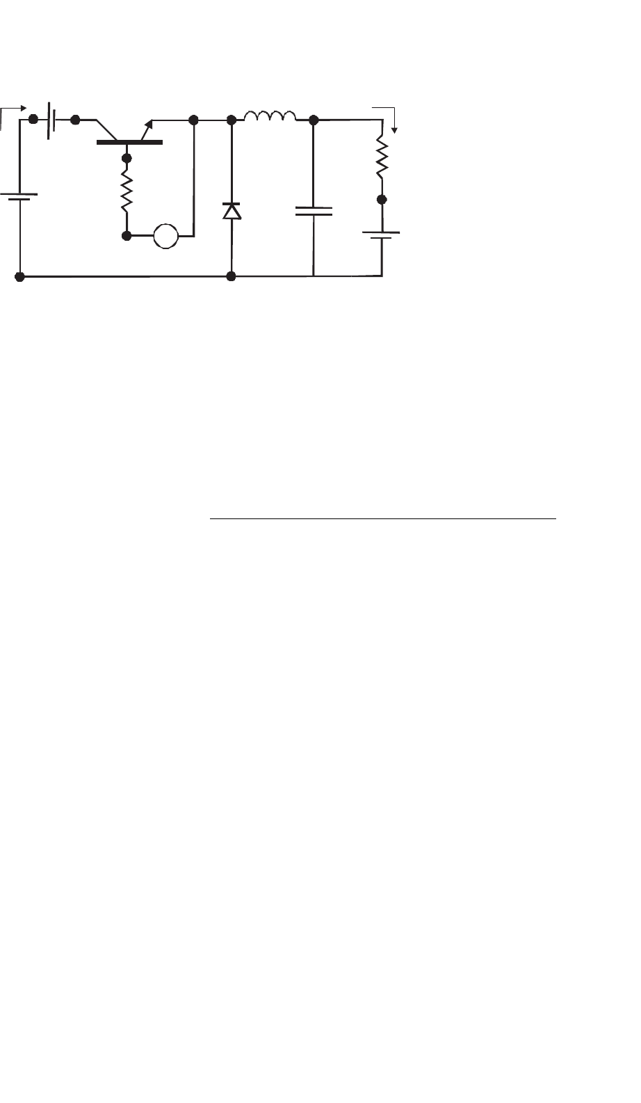
Figure 3.23 shows a BJT buck chopper. The dc input voltage

is 12 V, the load resistance R is 5 , the ﬁlter inductance L is

145.84 µH, and the ﬁlter capacitance C is 200 µF. The chop-

ping frequency is 25 kHz and the duty cycle of the chopper is

42% as indicated by the control voltage statement (V

). The

listing below plots the instantaneous load current (I

), the

input current (I

), the diode voltage (V

), the output voltage

), and calculate the Fourier coefﬁcients of the input cur-

rent (I

). It is suggested for the careful reader to have more

details and enhancements on using SPICE for simulations on

specialized literature and references.

*SOURCE

VS 1 0 DC 12V

VY 1 2 DC 0V ;Voltage source to measure

input current

VG 7 3 PULSE 0V 30V 0.1NS 0/1Ns 16.7US 40US)

*CIRCUIT

RB 7 6 250 ;Transistor base

resistance

R505

L 3 4 145.8UH

C 5 0 200UF IC=3V ;Initial voltage

VX 4 5 DC 0V ;Source to inductor

current

DM 0 3 DMOD ;Freewheeling diode

.MODEL DMOD D(IS=2.22E–15 BV=1200V CJO=O TT=O)

Q126332N6546 ;BJT switch

.MODEL 2N6546 NPN (IS=6.83E–14 BF=13 CJE=1PF

CJC=607.3PF TF=26.5NS)

*ANALYSIS

.TRAN 2US 2.1MS 2MS UIC ;Transient analysis

.PROBE ;Graphics post-processor

.OPTIONS ABSTOL=1.OON RELTOL=0.01 VNTOL=0.1

ITL5=40000

.FOUR 25KHZ I (VY) ;Fourier analysis

.END

3.7 BJT Applications

Bipolar junction power transistors are applied to a variety

of power electronic functions, switching mode power sup-

plies, dc motor inverters, PWM inverters just to name a few.

To conclude the present chapter, three applications are next

illustrated.

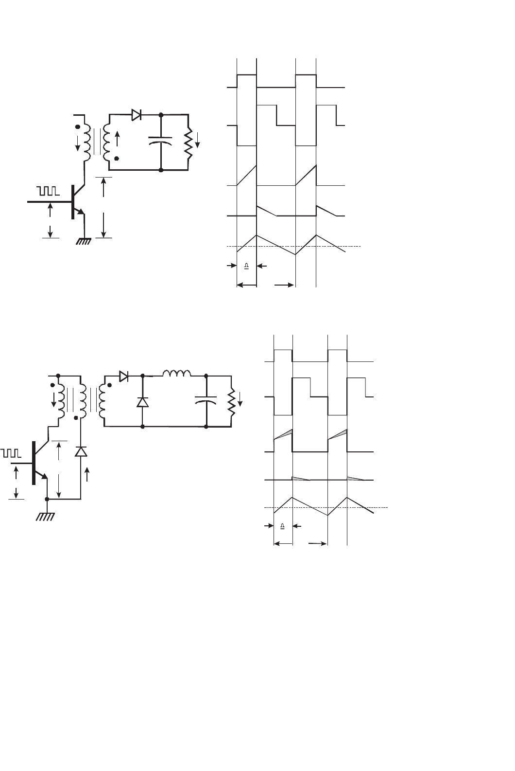
A ﬂyback converter is exempliﬁed in Fig. 3.24. The switching

transistor is required to withstand the peak collector voltage

at turn-off and peak collector currents at turn-on. In order to

limit the collector voltage to a safe value, the duty cycle must be

kept relatively low, normally below 50%, i.e. 6. < 0.5. In prac-

tice, the duty cycle is taken around 0.4, which limits the peak

collector. A second design factor which the transistor must

meet is the working collector current at turn-on, dependent

on the primary transformer-choke peak current, the primary-

to-secondary turns ratio, and the output load current. When

the transistor turns on the primary current builds up in the

primary winding, storing energy, as the transistor turns off,

the diode at the secondary winding is forward biasing, releas-

ing such stored energy into the output capacitor and load.

Such transformer operating as a coupled inductor is actually

deﬁned as a transformer-choke. The design of the transformer-

choke of the ﬂyback converter must be done carefully to avoid

saturation because the operation is unidirectional on the B–H

characteristic curve.

Therefore, a core with a relatively large volume and air gap

must be used. An advantage of the ﬂyback circuit is the sim-

plicity by which a multiple output switching power supply may

38 M. G. Simoes

On Off On

OUT

FIGURE 3.24 Flyback converter.

On Off On

OUT

FIGURE 3.25 Isolated forward converter.

be realized. This is because the isolation element acts as a com-

mon choke to all outputs, thus only a diode and a capacitor

are needed for an extra output voltage.

Figure 3.25 shows the basic forward converter and its

associated waveforms. The isolation element in the forward

converter is a pure transformer which should not store energy,

and therefore, a second inductive element L is required at the

output for proper and efﬁcient energy transfer. Notice that

the primary and secondary windings of the transformer have

the same polarity, i.e. the dots are at the same winding ends.

When the transistor turns on, current builds up in the pri-

mary winding. Because of the same polarity of the transfo

rmer secondary winding, such energy is forward transferred

to the output and also stored in inductor L through diode D

which is forward-biased. When the transistor turns off, the

transformer winding voltage reverses, back-biasing diode D

3 Power Bipolar Transistors 39

FIGURE 3.26 Chopper-fed dc drive.

and the ﬂywheel diode D

is forward-biased, conducting

current in the output loop and delivering energy to the load

through inductor L. The tertiary winding and diode D, provide

transformer demagnetization by returning the transformer

magnetic energy into the output dc bus. It should be noted

that the duty cycle of the switch must be kept below 50%,

so that when the transformer voltage is clamped through the

tertiary winding, the integral of the volt-seconds between the

input voltage and the clamping level balances to zero. Duty

cycles above 50%, i.e. 6 > 0.5, will upset the volt-seconds bal-

ance, driving the transformer into saturation, which in turn

produces high collector current spikes that may destroy the

switching transistor. Although the clamping action of the ter-

tiary winding and the diode limit the transistor peak collector

voltage to twice the dc input, care must be taken during con-

struction to couple the tertiary winding tightly to the primary

(biﬁlar wound) to eliminate voltage spikes caused by leakage

inductance.

Chopper drives are connected between a ﬁxed-voltage dc

source and a dc motor to vary the armature voltage. In addition

to armature voltage control, a dc chopper can provide regener-

ative braking of the motors and can return energy back to the

supply. This energy-saving feature is attractive to transporta-

tion systems as mass rapid transit (MRT), chopper drives are

also used in battery electric vehicles. A dc motor can be oper-

ated in one of the four quadrants by controlling the armature

or ﬁeld voltages (or currents). It is often required to reverse

the armature or ﬁeld terminals in order to operate the motor

in the desired quadrant. Figure 3.26 shows a circuit arrange-

ment of a chopper-fed dc separately excited motor. This is a

one-quadrant drive, the waveforms for the armature voltage,

load current, and input current are also shown. By varying the

duty cycle, the power ﬂow to the motor (and speed) can be

controlled.