Pao Y.C. Engineering Analysis: Interactive Methods and Programs with FORTRAN, QuickBASIC, MATLAB, and Mathematica

Подождите немного. Документ загружается.

Beam Deﬂection Problem

MATHEMATICA APPLICATIONS

For solving the membrane problem, Mathematica can be applied as follows:

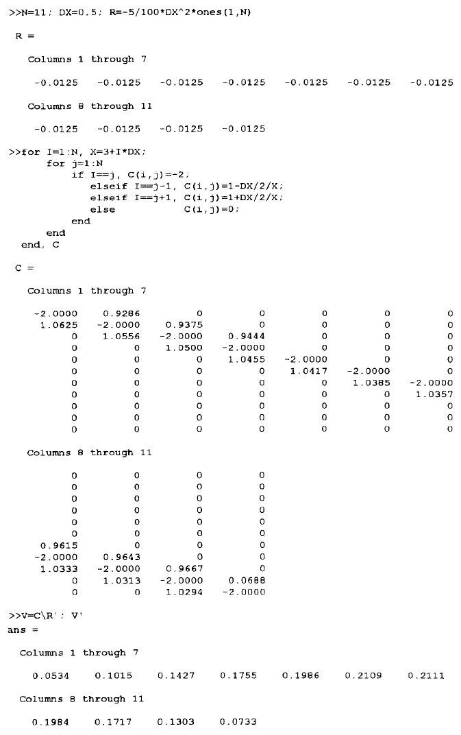
In[1]: = Ns = 11; DX = 0.5; c = Table[0,{Ns},{Ns}];

R = Table[–5*DX^2/100,{Ns}];

Print[“R = “,R]

Out[1] = R = {–0.0125, –0.0125, –0.0125, –0.0125, –0.0125, –0.0125,

–0.0125, –0.0125, –0.0125, –0.0125, –0.0125}

In[2]: = (Do[Do[x = 3 + i*DX; If[i = = j, c[[i,j]] = –2;,

If[i = = j–1, c[[i,j]] = 1DX/2/x;,

If[i = = j + 1, c[[i,j]] = 1 + DX/2/x;, Continue]]],

{i,Ns}], {j,Ns}]); Print[“Matrix c = “,c]

Out[2] = Matrix c = {{–2, 0.928571, 0, 0, 0, 0, 0, 0, 0, 0, 0},

{1.0625,–2, 0.9375, 0, 0, 0, 0, 0, 0, 0, 0},

{0, 1.05556, –2, 0.944444, 0, 0, 0, 0, 0, 0, 0},

{0, 0, 1.05, –2, 0.95, 0, 0, 0, 0, 0, 0},

{0, 0, 0, 1.04545, –2, 0.954545, 0, 0, 0, 0, 0},

{0, 0, 0, 0, 1.04167, –2, 0.958333, 0, 0, 0, 0},

{0, 0, 0, 0, 0, 1.03846, –2, 0.961538, 0, 0, 0},

{0, 0, 0, 0, 0, 0, 1.03571, –2, 0.964286, 0, 0},

{0, 0, 0, 0, 0, 0, 0, 1.03333, –2, 0.966667, 0},

{0, 0, 0, 0, 0, 0, 0, 0, 1.03125, –2, 0.96875},

{0, 0, 0, 0, 0, 0, 0, 0, 0, 1.02941, –2}}

In[3]: = V = Inverse[c].R

Out[3] = {0.0533741, 0.101498, 0.142705, 0.175525, 0.198641, 0.210864,

0.211107, 0.198368, 0.171723, 0.13031, 0.0733212}

These results are in agreement with those obtained by the MATLAB application.

The loaded beam problem also can be treated in a similar manner as follows:

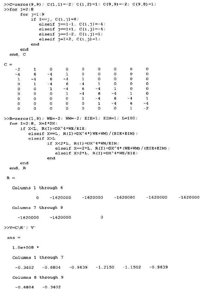
In[1]: = c = Table[0,{9},{9}]; c[[1,1]] = –2; c[[1,2]] = 1; c[[9,9]] = –2;

c[[9,8]] = 1;

In[2]: = (Do[Do[If[i = = j,c[[i,j]] = 6;, If[(j = = i–1)||(j = = i + 1), c[[i,j]] = –4;,

If[(j = = i + 2)||(j = = i–2), c[[i,j]] = 1;, Continue]]],

{i,2,8}],{j,9}]); Print[“Matrix c = “,c]

Out[2] = Matrix c = {{–2, 1, 0, 0, 0, 0, 0, 0, 0}, {–4, 6, –4, 1, 0, 0, 0, 0, 0},

{1, –4, 6, –4, 1, 0, 0, 0, 0}, {0, 1, –4, 6, –4, 1, 0, 0, 0},

{0, 0, 1, –4, 6, –4, 1, 0, 0}, {0, 0, 0, 1, –4, 6, –4, 1, 0},

{0, 0, 0, 0, 1, –4, 6, –4, 1}, {0, 0, 0, 0, 0, 1, –4, 6, –4},

{0, 0, 0, 0, 0, 0, 0, 1, –2}}

In[3]: = R = Table[0,{9}]; WE = –2; WM = –2; EIE = 1; EIM = 1; L = 100;

DX = 30;

In[4]: = (Do[X = i*DX; If[X<L, R[[i]] = DX^4*WE/EIE;,

If[X = = L, R[[i]] = DX^4*(WE + WM)/(EIE + EIM);,

If[X>L, If[X<2*L, R[[i]] = DX^4*WM/EIM;,

If[X = = 2*L, R[[i]] = DX^4*(WE + WM)/(EIE + EIM);,

IF[X>2*L, R[[i]] = DX^4*WE/EIE;,

Continue]]]]]],

{i,2,8}]); Print[“R = “,R]

Out[4] = R = {0, –1620000, –1620000, –1620000, –1620000, –1620000,

–1620000, –1620000, 0}

In[5]: = V = Inverse[c].R

Out[5] = {–34020000, –68040000, –96390000, –115020000, –121500000,

–115020000, –96390000, –68040000, –34020000}

Again, the results are in agreement with those obtained by the MATLAB

application.

6.5 PROBLEMS

UNGEKUT

1. The differential equation of motion of a spring-and-mass system is d

x/dt

+ ω

x = 0 where ω

= k/m, m is the mass and k is the spring constant. If

the weight is 5 lb., g = 32.2 ft/sec

, k = 1.5 lb/in, and initially the dis-

placement x = 2 in. and velocity dx/dt = 0, use the 4th-order Runge-Kutta

method and a step-size of 0.05 sec. to manually calculate the values of x

and dx/dt at t = 0.05 sec. Note that the given second-order ordinary

differential equations should ﬁrst be converted into two ﬁrst-order differ-

ential equations.

2. Initially, the two functions x(t) and y(t) have values 1 and –1, respectively.

That is x(t = 0) = 1 and y(t = 0) = –1. For t>0, they satisfy the differential

equations dx/dt = 5x–2y + 2t and dy/dt = x

–0.25sin2t. Use Runge-Kutta

classic fourth-order method and a time increment of 0.01 second to cal-

culate x(t = 0.01) and y(t = 0.01).

3. In the following two equations, the terms dx/dt and dy/dt both appear.

2dx/dt –3x + 5dy/dt –7y = .5t + 1

–3dx/dt -x – 4dy/dt + 9y = .2e

–3t

Separate them by treating them as unknowns and solve them by simple

substitution or Cramer’s rule. The resulting equations can be expressed

in the forms of dx/dt = F

(t,x,y) and dy/dt = F

(t,x,y). Carry out by manual

computation using Runge-Kutta method to obtain the x and y values when

t = 0.1 if the time increment is 0.1 and the initial conditions are x(t = 0) =

1 and y(t = 0) = –2.

4. The distributed loads on the beam shown in Figure 3 can be described as

w = –1 N/cm, for 0<x<10 cm; w = 2.2x N/cm, for 10<x<20 cm; w = 0,

for 20<x<40 cm. Meanwhile, the bending moment applied at x = 30 cm

can be described as M

= 0, for 0<x<30 cm and M

= –3 N-cm, for

30<x<40 cm. By introducing new variables t, and x

through x

so that

t = x, x

= y, x

= dy/dx, x

= d

y/dx

, and x

= d

y/dx

, the problem of

ﬁnding the deﬂection y(x) of the beam can be formulated (see the refer-

ence cited in footnote) as:

/dt = F

(t,x

) = x

, x

(t = 0) = 0

/dt = F

(t,x

) = (x

+ M

)/EI, x

(t = 0) = 0

/dt = F

(t,x

) = x

, x

(t = 0) = –1121/3

/dt = F

(t,x

) = w, x

(t = 0) = 24

with M

and w being the applied bending moment and distributed loads,

respectively. The initial conditions speciﬁed above are all at the left end

of the beam which is built into the wall and for the deﬂection (x

), slope

), bending moment (x

), and shearing force (x

), respectively. Apply

the program RungeKut by using EI = 2x10

N/cm

and various stepsizes

to tabulate the results and errors similar to that given in the text.

5. Apply the fourth-order Runge-Kutta method to ﬁnd the values of x

and

at the time t = 0.2 second using a time increment of 0.1 second based

on the following governing equations:

At t = 0.1 second, x

= –1 and x

= 1.

6. Use different stepsizes to calculate y values at x = 0.1, 0.2, and 0.3 by

application of the program RungeKut for the initial-value problem

dy/dx = x

–y, y(x = 0) = 1. The analytical solution is y = 2–2x + x

-x

, by

which the exact solutions can be easily computed to be y(0.1) = 0.90516,

y(0.2) = 0.82127, and y(0.3) = 0.74918. Determine the stepsize which will

lead to a Runge-Kutta numerical solutions of y(0.1), y(0.2), and y(0.3)

accurate to ﬁve decimal ﬁgures.

7. For the loaded beam shown in Figure 13, the deﬂection y(x) is to be

determined by solving Equation 21. Let the stiffness EI be equal to 2x10

N-cm

and it can be shown that the bending moment M can be described

by the equations:

x x t and

xxx e

112

45 7 2 3 6=− + − =− + +

−

M = -x

+ 180x–9600 for 0<x<40 cm

and

M = 100x–8000 for 40<x<80 cm

Apply the program RungeKut to ﬁnd y at x = 80 cm by using stepsizes

h = 4, 2, 1, 0.5, 0.25, and 0.1 and calculate the error by comparing with

the expected value of y(x = 80) = –0.928 cm.

8. Convert the following two differential equations into three ﬁrst-order

differential equations in the forms of dx

/dt = F

(t;x

;constants) for

i = 1,2,3 so that the subroutine RKN can be readily applied:

9. Write a subprogram FUNCTION F(X,T,I,N) which includes the statements

COMMON R1,R2,R3,R4

for transmitting the values of R1, R2, R3, and R4 from the main program.

These four variables are r

, r

, and r

, respectively, appearing in the

equations:

FIGURE 13. Question 7.

uv t

uv e

23450670

0 1 20 300 0

+++−− =

−+− =

−

. sin

rA rB

rB rC

=−

This FUNCTION is to be used by the subroutine RKN in application of

the fourth-order Runge-Kutta method.

10. The functions x(t) and y(t) satisfy the differential equations d

x/dt

3dx/dt + 5dy/dt–7e

–9t

+ 9sin2t = 0 and 2dx/dt–4dy/dt + 6x–8y + 10t–12 =

0. Convert the above two equations into the standard form dx

/dt = f

(t;

;constants) for i = 1,2,3 where x

= x, x

= y, and x

= dx/dt. Give

the expressions for f

, f

, and f

in terms of t, x

, x

, and x

so that the

Runge-Kutta method can be applied.

11. Apply the fourth-order Runge-Kutta method to ﬁnd the values of y and

z at x = 0.35 if at x = 0.3, y = 1 and z = 2 respectively and they satisfy

thedifferential equations dy/dx = xy + z and dz/dx = yz + x. Use a stepsize

of x = 0.5 and show all details of how the Runge-Kutta parameters are

calculated.

12. The deﬂection y of the load beam shown below satisﬁes the ordinary

differential equation EI(d

y/dx

) = M where the Young’s modulus E =

2x10

N/m

, moment of inertia I = 4.5x10

–8

and the internal bending

moment, in N-m, has been derived in terms of x as M(x) = 200x–30 for

0≤x≤.1 m and M(x) = 100x–20 for .1≤x≤.2 m. (1) Using an increment of

x = 0.01 m, standardize the above problem into a system of two ﬁrst-

order ordinary differential equations dx

/dx = f

(x;x

;constants) for i =

1,2 where x

= y and x

= dy/dx (slope). (2) Write a FUNCTION F(…)

needed in SUBROUTINE RKN which we have discussed in class for

using the fourth-order Runge-Kutta method, based on the result of Step

(1) and also the M(x) equations. (3) Calculate the eight RungeKutta

parameters and then the value of y and dy/dx at x = 0.01 m.

13. Convert the following differential equation into a set of two ﬁrst-order

differential equations so that the fourth-order Runge-Kutta method can

be applied: d

x/dt

+ 4dx/dt + 3x = 4e

-t

. If at t = 0, x = 0 and dx/dt = 2,

use a time increment oft = 0.1, compute the x and dx/dt values at t =

0.1 based on the fourth-order Runge-Kutta method.

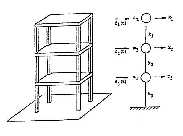
14. The forced swaying motion of a three-story building can be simulated as

a system of three lumped masses m

connected by springs with stiffnesses

and subjected to forces f

(t) for i = 1,2,3 as shown in Figure 14. Here,

the dampingcharacteristics are not considered but could be incorporated.

Derive the governing differential equations for the and then convert them

into a system of 6 ﬁrst-order differential equations so that the programs

RungeKut and ode45 can be applied to ﬁnd the histories of displace-

ments, x

(t), and velocities v

(t) = dx

(t)/dt. Solve a numerical case of m

2i N-sec

/cm, k

= 3i N/cm, and f

(t) = (2i–3)sin(2i–1)t N, x

(t = 0) = 0

and v

(t = 0) = 0 for 0<t≤20 seconds. Plot all displacement and velocity

histories.

rC rD

=−

15. Instead of f(t) = 1 in obtaining the system’s response of the mechanical

vibration problem using the MATLAB ﬁle FunMCK.m shown in

Figure 5, resolve the problem for the case of f(t) = 5sin(0.5t–0.3) by

changing FunMCK.m and plot the resulting displacement and velocity.

16. Implement the Runge-Kutta solution of Equation 30 by deﬁning a sub-

program function TwoMs in FORTRAN, QuickBASIC, or, MATLAB

to obtain the result shown in Figure 5 for the case of b = 3.6 m, h = 1.5

m, m

= 0.8, and initial conditions y = z = dy/dt = dz/dt = 0. And

calculate the histories of the cable tension T(t) and angle (t).

17. For the nonlinear oscillation problem of two connected masses shown in

Figures 4 and 5, we observe that the oscillation goes on continuously. The

motion can be damped by adding a viscous device vertically connected

to the mass whose displacement is denoted as z(t). This could be a

frictional wall, on which the mass slides vertically. Usually, the retarding

force of such a damping device, F

, could be assumed to be linearly

proportional to the velocity of the motion, dz/dt. That is, F

= cdz/dt where

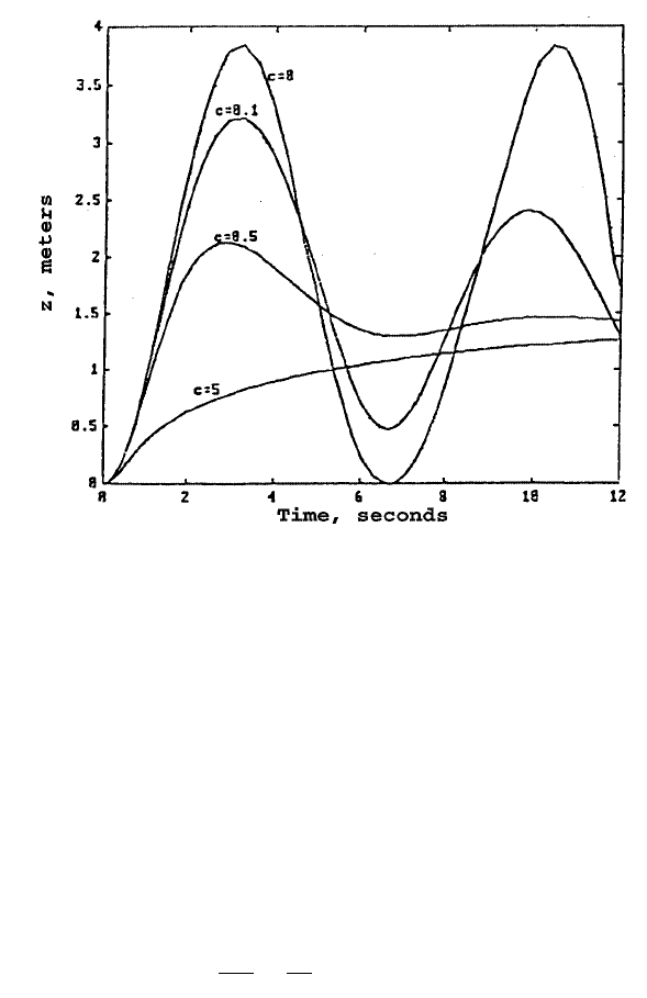
c is constant. Figure 15 is a result of the oscillation when a damping

device having c = 1 N-sec/m and m

= 1 N-sec

/m is added to that system.

We notice that amplitudes of y(t) and z(t) shown in Figure 5 are steadily

decreased. Develop this modiﬁed program in FORTRAN, QuickBASIC,

or,MATLAB to generate Figure 15.

18. Use Mathematica’s function NDSolve to solve Problem 7.

FIGURE 14. Problem 14.

19. Apply Mathematica to solve Problem 17 for a time increment t = 0.2

sec and until t = 12 seconds.

20. Apply Mathematica for solving Problem. 14.

ODEBVPRK

1. The function y(x) satisﬁes the boundary conditions y(x = 0) = 2 and y(x =

3) = 4 and the differential equation 5d

y/dx

–3dy/dx + y = 13x–15 for

0<x<3. Apply the fourth-order Runge-Kutta method to ﬁnd the y values

at x = 1 and x = 2 based on an increment of x equal to 1.

2. The function y(x) has the boundary values of y(x = 0) = 1 and y(x = 3) = 5

and for x between 0 and 3, y(x) satisﬁes the ordinary differential equation:

Apply the fourth-order Runge-Kutta method to ﬁnd the y values at x = 1

and x = 2 based on a stepsize of x = 1.

3. For a membrane (Figure 16) under uniform tension T and fastened at the

inner radius R

and outer radius R

, the axisymmetric deformation z

resulted by the acting uniform pressure p can be shown to satisfy the

differential equation:

FIGURE 15. Problem 17.

3221−+=+

for R

<r<R

. The boundary conditions are z(R

) = 0 and z(R

) = 0. Modify

the program OdeBvpRK to solve this problem.

4. A cable hung at its two ends as shown in Figure 17 by its own weight

will have a catenary shape described by the equation:

FIGURE 16. Problem 3.

FIGURE 17. Problem 4.

dr r

+=−