Pao Y.C. Engineering Analysis: Interactive Methods and Programs with FORTRAN, QuickBASIC, MATLAB, and Mathematica

Подождите немного. Документ загружается.

Output[1] =

m = {{0,2,3), {–10,–1,2}, {–2,4,7}}

Notice that the elements in each row are separated by comma and enclosed by

a pair of braces, and rows are separated also by comma. Next, we derive the

characteristic equation of the matrix m.

Input[2]: =

Det[m — x IdentityMatrix[3]]

Output[2] =

6 – 11 X + 6 X

— X

Input[3]: =

m = {{1,2,3), {–10,0,2}, {–2,4,8}}

Output[3] =

m = {{1,2,3), {–10,0,2}, {–2,4,8}}

Input[4]: =

Det[m — x IdentityMatrix[3]]

Output[4] =

24 – 26 X + 9 X

– X

We may proceed to solve the characteristic roots as follows:

Input[5]: =

NSolve[24–26x + 9x^2x^3 = = 0,x]

Output[5] =

{{x -> 2.}, {x -> –3.}, {x -> 4.}}

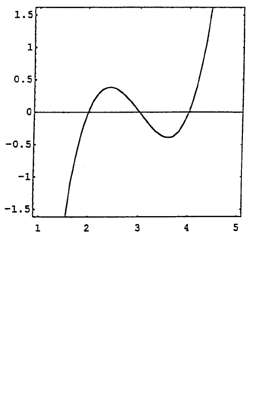
Again, the polynomial can be plotted with:

Input[6]: =

Plot[x^3–9x^2 + 26x–24, {x,1,5},

Frame->True}, AspectRatio->1]

Output[6] =

Notice that the graph intercepts the x axis at x = 2, x = 3, and x = 4.

7.4 PROGRAM EIGENVEC — SOLVING EIGENVECTOR

BY GAUSSIAN ELIMINATION METHOD

The program EigenVec is designed to solve for the associated eigenvector {V} when

an eigenvalue of a given square matrix [A] is speciﬁed. Eigenvalue and eigenvector

problems are discussed in the programs CharacEq and EigenODE. Here, we

describe how the Gaussian Elimination method can be modiﬁed for ﬁnding the

eigenvector {V}. Since the eigenvector {V} satisﬁes the matrix equation:

(1)

where [I] is the identity matrix of same order as [A]. Equation 1 is called homoge-

neous since the right-hand side is a null vector. This equation has nontrivial solution

only if the determinant of the coefﬁcient matrix [A]–[I] is equal to zero. In other

words, the linear algebraic equations represented by Equation 1 are not all indepen-

dent. The number of equations which are dependent on the other equations, is equal

to the multiplicity of the speciﬁed . For example, if the matrix [A] is of order N

and if the multiplicity of  is M which means M characteristic roots are equal to ,

then there are M equations in Equation 1 are dependent on the other N-M equations.

AIV

[]

−

[]

()

{}

λ 0

When Gaussian Elimination method is applied for solving {V} from Equation

1, the normalization of the last equation cannot be carried out if  has a multiplicity

equal to 1 even with the pivoting provision in the program. This is because one of

the N equation is dependent on the other N–1 equations. But, it suggests that we

may assign the last component of {V} to be equal to an arbitrary constant c and

express the other components of {V} in terms of c. This concept can be extended

to the case when λ has a multiplicity of M. Since only N-M equations of (1) are

independent, there are M independent solutions of {V}. To obtain the ﬁrst solution,

we assign the last component of {V} a value c

and the other last M–1 components

of {V} equal to zero and then proceed to express the ﬁrst N-M components of {V}

in terms of c

. To obtain the second solution, we assign the next to the last component

of {V} a value c

and the other last M–1 components of {V} equal to zero and

express the ﬁrst N-M components of {V} in terms of c

, and so on. The M solution

of {V} can thus be expressed in terms of c

for i = 1,2,…,M.

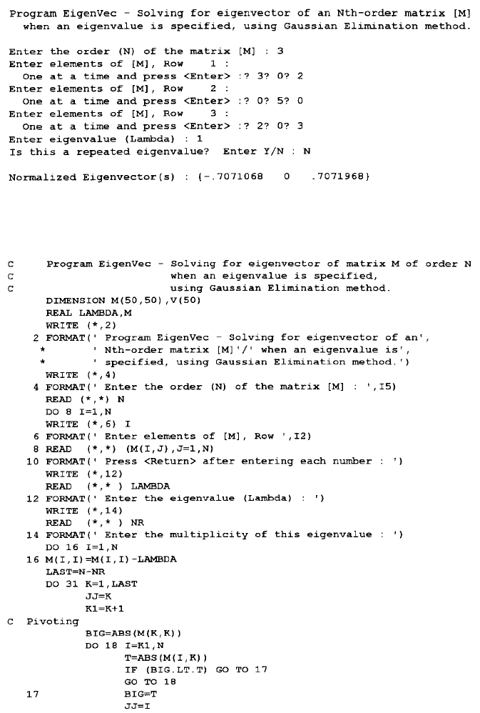
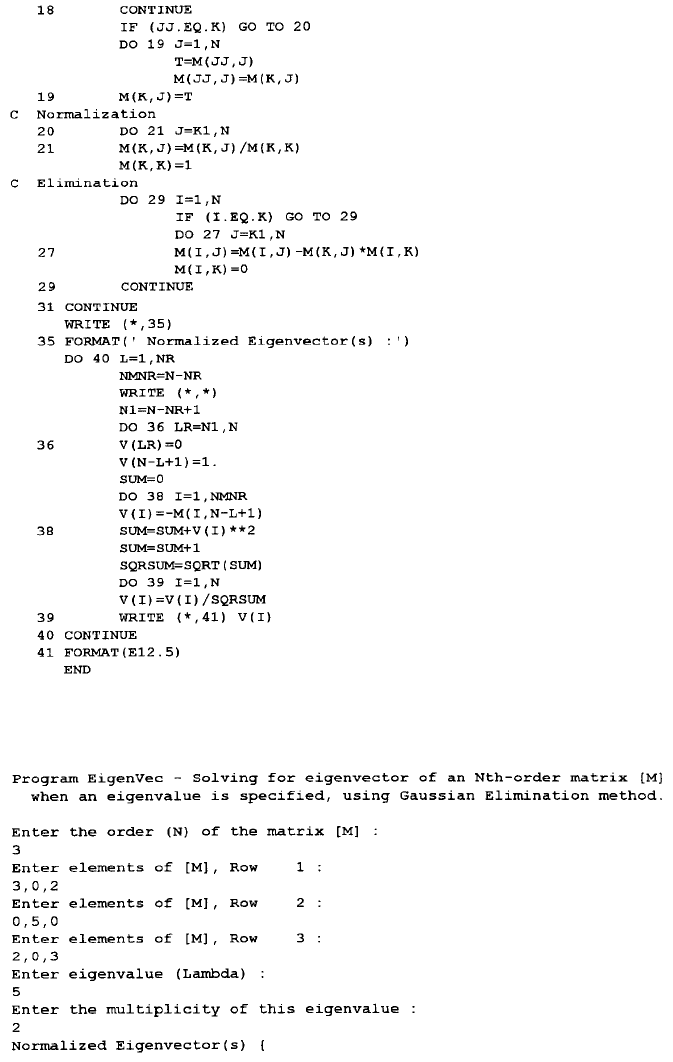
The program EigenVec is developed from modifying the program Gauss by

following the above-explained procedure. This program requires the user to inter-

actively specify the order N of [A], the elements of [A], a speciﬁed value of  and

its multiplicity M. The results produced by the program EigenVec are the M set of

eigenvectors {V}. Both FORTRAN and QuickBASIC versions of this programs are

listed below along with sample applications.

QUICKBASIC VERSION

Sample Application

FORTRAN VERSION

Sample Application

MATLAB APPLICATIONS

MATLAB has a ﬁle called eig.m which can be applied for ﬁnding the eigen-

values and normalized vectors of a speciﬁed square matrix. To do so, we ﬁrst

interactively specify the elements of a matrix [A} and then ask for the eigenvalues

Lambda and normalized eigenvectors EigenVec by entering (such as for the sample

problem in the FORTRAN and QuickBASIC versions)

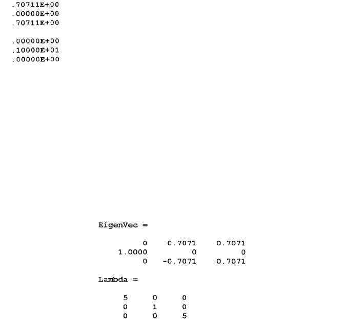
>> A = [3,0,2;0,5,0;2,03]; [EigenVec,Lambda] = eig(A)

It results in a display on the screen:

Notice that the eigenvalues are listed in the diagonal of the matrix Lambda and

the corresponding normalized eigenvectors are listed in the matrix EigenVec as

columns. To list the eigenvalues in a vector Lambda, we could enter:

>> [Lambda] = eig(A)

The resulting display is:

Lambda =

MATHEMATICA APPLICATIONS

Mathematica has functions Eigenvalues and Eigenvectors which can be

applied to ﬁnd the eigenvalues and eigenvectors, respectively, for a speciﬁed matrix

as illustrated by the following example:

In[1]: = a = {{3,0,2},{0,5,0},{2,0,3}}; MatrixForm[a]

Out[1]//MatrixForm: =

302

050

203

In[2]: = Eigenvalues[a]

Out[2]: =

{1, 5, 5}

In[3]: = Eigenvectors[a]

Out[3]: =

{–1, 0, 1}, {1, 0, 1}, {0, 1, 0}}

Notice that the computed eigenvectors are not normalized.

As another example, consider the matrix M generated in the program EigenODE

for the buckling problem when the number of stations is equal to 5. To obtain the

eigenvalues, the interactive application of Mathematica goes as:

In[4]: = Eigenvalues[M]

Out[4]: =

{134.354, 108., 72., 36., 9.64617}

Notice that the smallest eigenvalue is equal to 9.64617 which predicts the lowest

buckling load. Since the exact solution is 9.8696, this further indicates that by

continuously increasing the number of stations the smallest eigenvalue in magnitude

will eventually converge to the expected value.

PRINCIPAL STRESSES AND PLANES

As another example of solving the eigenvalues and eigenvectors, consider the

problem of determining the principal stresses at a point within a two-dimensional

body which is subjected to in-plane loadings. If the normal stresses (

and σ

) and

shear stresses (

= 

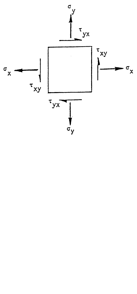
), Figure 5, at that point are known, it is a common practice

to graphically determine the principal stresses and principal planes, on which the

principal stresses act by use of Mohr’s circle.

But, here we demonstrate how the

principal stresses and principal planes can be solved as the eigenvalues and eigen-

vectors, respectively, of a matrix [A] constructed using the values of 

, 

, and 

as follows:

(2)

For the three-dimensional cases, the normal stresses 

, 

, and 

, and shear

stresses 

, 

, and 

(

= 

, 

= 

, and 

= 

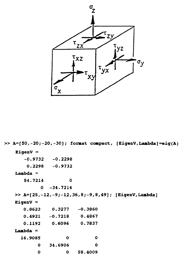
) are involved, Figure 6.

Again, the Mohr’s circle method can be applied to graphically solve for the principal

stresses and the principal planes, on which they act.

But, as an extension of Equation

2, these principal stresses and principal planes can be determined as the eigenvalues

and eigenvectors, respectively, of a matrix constructed using the values of the normal

and shear stresses as follows:

(3)

Presented below are MATLAB solutions of two problems: (a) a two-dimensional

case of 

= 50, 

= –30, and 

= 

= –20, and (b) a three-dimensional case of



= 25, 

= 36, 

= 49, 

= 

= –12, 

= 

= 8, and 

= 

= –9, all in N/cm

FIGURE 5. If the normal stresses (

and σ

) and shear stresses (

= 

), are known, it

is a common practice to graphically determine the principal stresses and principal planes, on

which the principal stresses act by use of Mohr’s circle.

xxy

yx y

[]













στ

τσ

xxyxz

yx y yz

zx zy z

[]













στ τ

τστ

ττσ

Notice that for Problem (a), the result indicates that maximum principal stress

equal to 54.7214 N/cm

is on a plane having an outward normal vector whose

directional cosines are equal to –0.9732 and 0.2298. That is to say this principal

plane has an outward normal vector making an angle of 

max

= 166.7° (cos

max

–0.9732 and cos[90°–

max

] = 0.2298) measured counterclockwise from the x-axis.

The minimum principal stress is found to be equal to –34.7217 N/cm

which is on

a plane having an outward normal vector whose directional cosines are equal to

–0.2298 and –0.9732, or at an angle equal to 

min

= –103.3° (cos

min

= 0.2298 and

FIGURE 6. For the three-dimensional cases, the normal stresses 

, 

, and 

, and shear

stresses 

, 

, and 

(

= 

, 

= 

, and 

= 

) are involved.

cos[90°– 

min

] = –0.9732). The two principal planes are perpendicular to each other.

This can also be proven by taking the dot product of the two normalized eigenvectors:

(–0.9732i + 0.2298j)•(–0.2298i- 0.9732j) = 0.

Similar observation can be made from the results for Problem (b). The principal

stresses are equal to 16.9085, 34.6906, and 58.4009 N/cm

and they on the planes

having outward normal vectors n

= 0.8632i + 0.4921j + 0.1192k, n

= 0.3277i –

0.7218j + 0.6096k, and n

= –0.3860i + 0.4867j + 0.7837k, respectively. It is easy

to prove that these principal planes are indeed orthogonal by showing that n

•n

= n

•n

= 0.

QUADRATIC FORMS AND CANONICAL TRANSFORMATION

Another interesting application of the procedure involved in solving eigenvalues

and eigenvectors of a square matrix is the canonical transformation of quadratic

forms

for Consider a surface described by the equation:

(4)

The left-hand side is called a quadratic form in x, y, and z. The surface is an

ellipsoid but it is difﬁcult to make out what are the values of its major and minor

axes, for which a transformation of the coordinate system is necessary for changing

the quadratic form into a canonical one. By canonical form, it means that only the

squared terms should remain. To ﬁnd what transformation is needed, we ﬁrst write

Equation 4 in matrix form as:

(5)

where:

(6,7)

It can be shown

that if we ﬁnd the eigenvalues and eigenvectors of [A] which

in fact are already available in the answer to the previously discussed Problem (b),

the coordinate system x-y-z can be transformed into another set of x-y-z system

by using the so-called normalized modal matrix, [Q], formed with the normalized

eigenvectors as its columns. That is:

(8)

25 36 49 24 18 16 100

222

xyzxyxzyz++−−+=

VAV

{}

[]

{}

=100

and A

{}













[]

−−

−













25 12 9

12 36 8

9849

′

{}

′













−

























[]

{}

.. .

...

.. .

8623 3277 3860

4921 7218 4867

1192 6096 7837