Pao Y.C. Engineering Analysis: Interactive Methods and Programs with FORTRAN, QuickBASIC, MATLAB, and Mathematica

Подождите немного. Документ загружается.

Because numerical differentiation is highly inaccurate, whenever possible

numerical integration should be preferred over numerical differentiation. In case that

one needs to ﬁnd the velocity of a certain motion study and has the option of

collecting the displacement or acceleration data, then the acceleration data should

be taken not the displacement data. The reason is that one has the choice of applying

numerical differentiation to the displacement data or numerical integration to the

acceleration data to obtain the velocity results. The numerical integration which is

the topic of Chapter 5 has the smoothing effect and hence is more accurate! Graph-

ically, differentiation is of a

local

evaluation of determining the slope at a selected

point on a curve which could be the result of ﬁtting a number of data points discussed

in Chapter 3 while integration is of a global evaluation of ﬁnding the area under the

curve between two speciﬁed limits of the independent variable. For a set of three

given points ﬁtted linearly by two linear segments and quadratically by a parabola,

the slope at the mid-point could have very different slope values while the areas

under the linear segments and under the parabola would not differ too signiﬁcantly.

Hence, it is worthy of emphasizing that learning the computational methods is easier

when compared to making decision of which method is best to solve the problem

at hand.

4.2 PROGRAM DIFFTABL — APPLICATIONS

OF FINITE-DIFFERENCE TABLE

Program

DiffTabl

has been developed for the need of constructing a table of ﬁnite

differences of a given set of N two-dimensional points, (x

) for i = 1–N. The x

values are assumed to be equally spaced, i.e., , x

–x

= x

–x

= ••• = x

-x

N–1

= h, h

being called the

increment

, or,

stepsize

. This so-called

difference table

can be applied

for interpolation of the y value for a speciﬁed, unlisted x value inside the range of

x = x

and x = x

(extrapolation if outside the range), and differentiation. Table 1

shows a typical difference table.

The symbol



used in Table 1 is called Forward Difference Operator. If we refer

the numbers listed in the x and y columns as x

to x

and y

to y

, respectively, the

ﬁrst number listed under



y, 1.9495, is obtained from the calculation of y

–y

and

is identiﬁed as

∆

. The last number listed in the



y column, 5.3015, is equal to

–y

and referred to as



. Or, we may write the general formula as, for i = 1 to 5,

(1)



is called the ﬁrst forward difference of y at x

. The higher order forward

differences listed in Table 1 are obtained by extended application of Equation 1.

That is,

(2)

∆yy y

ii i

=−

∆∆ ∆ ∆

1121

2yyyy yy yy

iiii ii ii

=−

()

=−=−+

++++

(3)

and so on. We shall show later how the third through seven columns of Table 1 can

be interpreted differently when the backward and central difference operators are

introduced. First, we will demonstrate how Table 1 can be applied for interpolation

of the y value at an unlisted x value, say y(x = 1.24). To do that, the

shifting operator

E, needs to be introduced. The deﬁnition of E is such that:

(4)

That is, if E is operating on y

, the y value is shifted down to the next provided

y value. Interpolation is a problem of not shifting a full step but a fractional step.

For the need of ﬁnding y at x = 1.24, the x value falls between x

= 1.2 and x

1.3. Since the stepsize, h, is equal to 0.1, a full shift from y

= 6.3760 would lead

to y

which is equal to 8.9625. We expect the value of y(x = 1.24) to be between y

and y

. Instead of E

, the value of E

0.4

is to be calculated by shifting only 40%.

To ﬁnd the meaning of E

0.24

, or, more generally E

for 0<r<1, we substitute

Equation 4 into Equation 1 to obtain:

(5,6)

TABLE 1

Difference Table (y = 1 to 2x + 3x

to 4x

+ 5x



1.1 4.4265

1.9495

1.2 6.3760 0.637

2.5865 0.126

1.3 8.9625 0.763 0.012

3.3495 0.138 0.000

1.4 12.3120 0.901 0.012

4.2505 0.150

1.5 16.5625 1.051

5.3015

1.6 21.8640

∆∆ ∆ ∆

321 21

321

yyyy y

yyyyyy

yyyy

iiii i

iiiiii

iiii

=−

()

=−

=− +

()

−−+

()

=− + −

+++++

+++

Ey y

∆yy yEyy E y

ii i ii

=−=−=−

()

∆∆=− =+EorE11, ,

By application of

binomial expansion

, we can then have:

(7)

where the binomial coefﬁcients are deﬁned as:

(8)

We can now use Equation 7 to obtain:

(9)

Equation 9 can be applied for linear interpolation if up to the



terms are

adopted; for parabolic interpolation if up to the



terms are adopted; and so on.

Since Table 1 has up to the ﬁfth order forward differences available but the last

column contains a zero value, Equation 9 can therefore be effectively up to the

fourth-order forward-difference interpolation. The numerical results of y(x = 1.24)

using linear, parabolic, cubic, and fourth-order are 7.4106, 7.3190, 7.3279, and

7.3274, respectively. Since we know y = 1–2x + 3x

–4x

+ 5x

, the exact value of

y(x = 1.24) is equal to 7.3274.

An explanation for discrepancies in all of these four attempts of interpolations,

relative to the exact value, is provided in a homework exercise given in the Problems

set.

ACKWARD

-D

IFFERENCE

PERATOR

Notice that the ﬁrst numbers listed in columns three through seven in Table 1

are the ﬁve forward differences of y

, and that only four forward differences (the

second numbers in columns three through six) of y

are available. Lesser and lesser

forward differences are available for later y’s until there is only



for y

. That is

to say, to interpolate y(x) for an x value between x

= 1.5 and x

= 1.6, Equation 9

can only be used up to the



term. To remedy this situation and to make most use

of the provided set of 6 (x,y) data, it is appropriate at this time to introduce the

backward-difference operator,



, which is deﬁned as:

(10)

()

∞

∑

∆∆

and

rr r k

()

−

()

…− −

()

[]

⋅

yx E yx E y y

()

==+

()

=+ +

−

()

⋅

+…













=+ − + − +

()

124 12 1

104

0404 1

1 0 4 1 12 0 064 0 0416 0 022952

04 04

23 4 5

.. . . .

∆

∆∆

∆∆ ∆ ∆ ∆

∇= −

−

yyy

iii1

By combining Equations 1, 7, and 10, we notice that:

(11)

and

(12)

So,

(13,14)

Equation 12 is an important result because it indicates that the last numbers

listed in columns three through seven of Table 1 are the ﬁrst through ﬁve backward

differences of y

. If we could derive an interpolation formula in terms of



, there

are up to ﬁfth-order backward difference of y

available. Toward that end, let us

consider the need of interpolating the value of y(x = 1.56). This y value can be

reached by shifting backward by 0.4 step from x = 1.6 since the stepsize for Table 1

is h = 0.1. By using Equation 14 and noticing Equations 7 and 8, we can have:

(15)

One can then apply Equation 15 to obtain the interpolated y(x = 1.56) values

using up to the ﬁfth order backward differences. This is left as a homework exercise

given in the Problems set.

ENTRAL

-D

IFFERENCE

PERATOR

For the interest of completeness and later application in numerical solution of

ordinary differential equations, we also introduce the

central difference operator



When it is operating on y

, the deﬁnition is:

(16)

The ﬁrst-order central difference is seldom used and the second-order central

difference is frequently applied, which is:

(17)

∇= −=

yyyy

iiii11

∆

∇= −=−

()

−+

−

yyy Ey

iii i11

∇= − = −∇

−−

EorE, ,

yx E yx E y y

()

==−∇

()

=+ −∇

()

−

()

⋅

−∇

()

+…













−−

156 16 1

104

0404 1

04 04

=− ∇− ∇− ∇− ∇− ∇

()

1 0 4 0 12 0 064 0 0416 0 02295

23 4 5

.. . . . y

δyyx

ii i









−−









δδ δ

yyx

yx h yx yx h

yyy

ii i i ii

iii





















−−





















()

−

()

+−

()

=−+

+−

IFFERENTIATION

PERATOR

Another important operator that needs to be introduced in connection with the

application of difference table is the

differentiation operator

, D, which is deﬁned as:

(18)

As it is our intention to apply an available difference table for numerical differ-

entiation at one of the listed x values, or, at an unlisted x value, by using either the

forward or backward differences of y values. For example, we may want to ﬁnd Dy

at x = 1.2, or, at x = 1.24. To derive an expression for D in terms of



, we recall

the Taylor’s series of a function y(x = a + h) near the neighborhood of x = a for a

small increment of h:

(19)

where y

(j)

is the jth derivative with respect to x. Using the notation of differentiation

operator D and the shifting operator E, the above expression can be written as:

(20)

or,

(21)

In order to use the difference table for numerical differentiation, we substitute

Equation 6 into Equation 21 to obtain:

(22)

By substituting the logarithmic function in Equation 21 with an inﬁnite series

and applying the D operator for y

, the result is:

(23)

Hence, to ﬁnd Dy(x = 1.2) by using the ﬁnite differences in Table 1, Equation

23 can be applied to obtain:

Dy x x

dy x

()

≡

()

≡

ya h ya

()

′

()

′′

()

+…+

()

+…

()

!! !

Ey a y a

hDy a h D y a h D y a

hD h D h D y a e y a

jj hD

()

+…+

()

+…

=+ + +…+ +…

[]

()

!! !

E e and D

n=+

()

1l ∆

=−+−…









∆∆ ∆

Notice that the above result is when up to the fourth-order forward differences

of y

are all utilized. Linear, parabolic, and cubic numerical differentiations at x =

1.2 could also be calculated by taking only one, two, and three terms inside the

parentheses of the above expression. The respective results are 25.865, 22.05, and

22.51. Since y(x) = 1–2x + 3x

2–

+ 5x

and y(x) = –2 + 6x–12x

+ 20x

, the exact

value of y(x = 1.2) = –2 + 7.2–17.28 + 34.56 = 22.48 indicates that the fourth-order

calculation is the best.

When Dy

is needed for x

near the end of x list, it is better to express D in terms

of the backward-difference operation , which based on Equations 14 and 21 is:

(24)

The shifting operator E and differentiation operator D can be combined to derive

formulas for numerical differentiation of y(x) at x values unlisted in the difference

table either in terms of forward-difference operator or backward-difference. First,

let recall Equations 7 and 23 and apply them to ﬁnd y(x = x

+ rh) in terms of the

forward-difference operator as follows:

(25)

Similarly, y(x

-rh) can be expressed in terms of backward-differential operator, as:

(26)

Dy x

2 5865 0 5 0 763

0 138

0 012 22 48=−+−









... . . .

Dy x

nEy

ii i

()

=−∇

()

[]

−

−∇ − ∇ − ∇ −…









=∇+

∇

+…













−

234

′

()

==+

()

=−+−…













−

()

+…













−

−+

−+−

yx rh

DE y

rrr rrr

121

362

2 9 11 3

l ∆∆

∆

∆∆

∆∆ ∆ ∆++…













′

−

()

==−−∇

()

[]

−∇

()

=∇+

∇

+…













−∇+

−

()

∇+…













=∇−

−

∇+

−+

∇−

−+−

−

yx rh

DE y

rrr rrr

121

362

2911

∇+…













It should be particularly pointed out that in using Equation 26 for ﬁnding y(x)

where x

i–1

<x<x

, r is to be calculated as (x

-x)/h and not as (x-x

i–1

)/h. For example,

in using Table 1, to calculate y(x = 1.56) based on Equation 26 r should be equal

to (1.6–1.56)/0.1 = 0.4 and not equal to (1.56–1.5)/0.1 = 0.6, and i equal to 6 not 5

because in Table 1 x

= 1.6 and x

= 1.5.

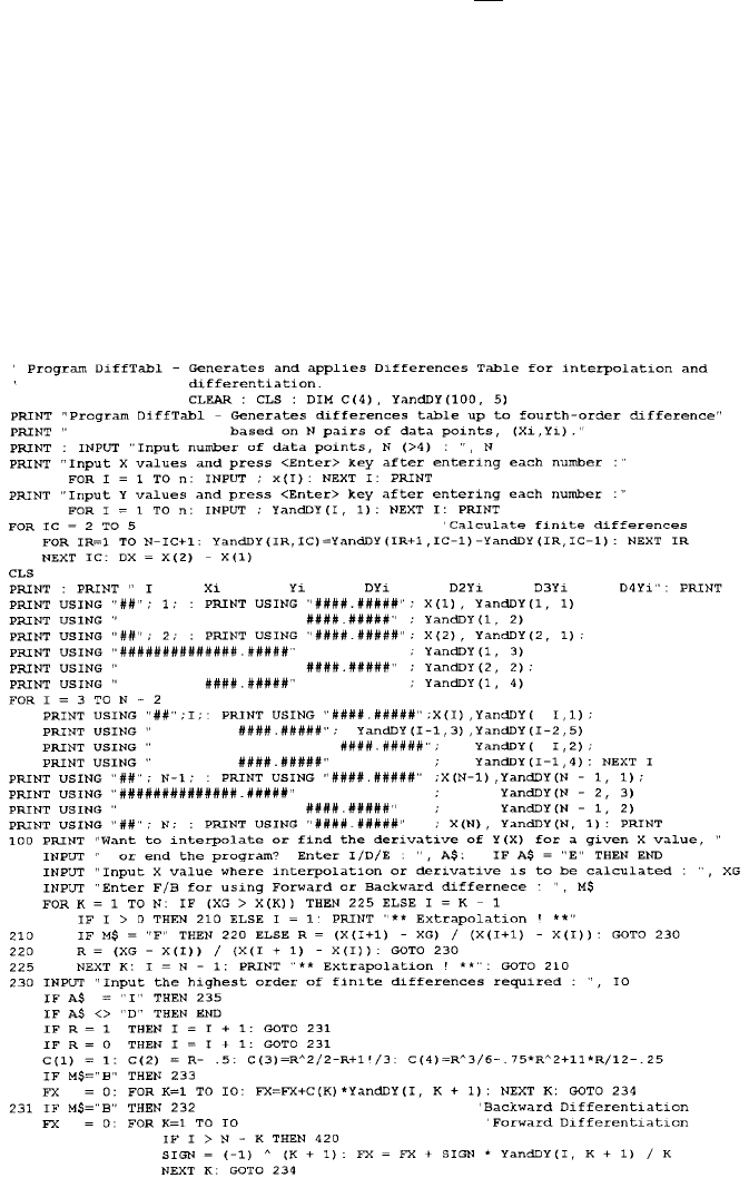
Program DiffTabl has been prepared for interactive interpolation and differen-

tiation using a difference table such as Table 1. User can interactively specify the

data points and where the interpolation or differentiation is to be calculated and also

up to what order of ﬁnite differences should the computation be performed. Both

QuickBASIC and FORTRAN versions of the program are made available. Listings

are given below along with some sample applications. At present, the highest order

of ﬁnite difference allowed is the fourth.

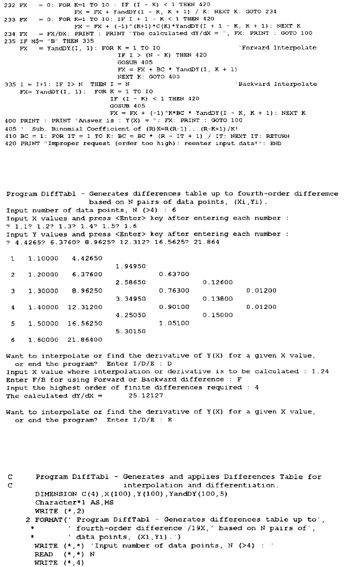
QUICKBASIC VERSION

Sample Application

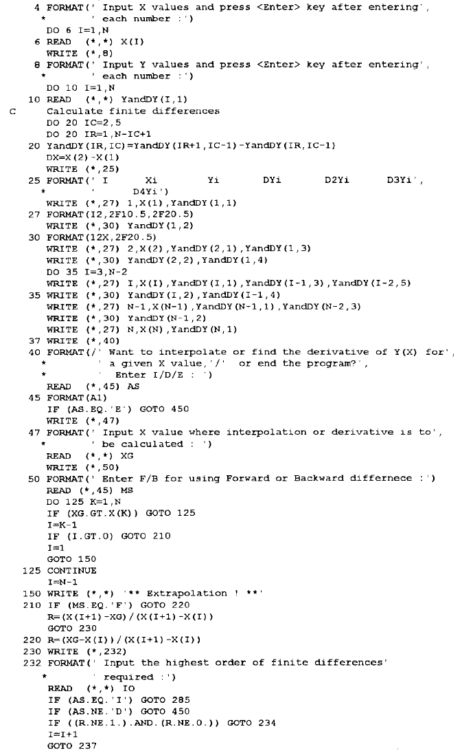
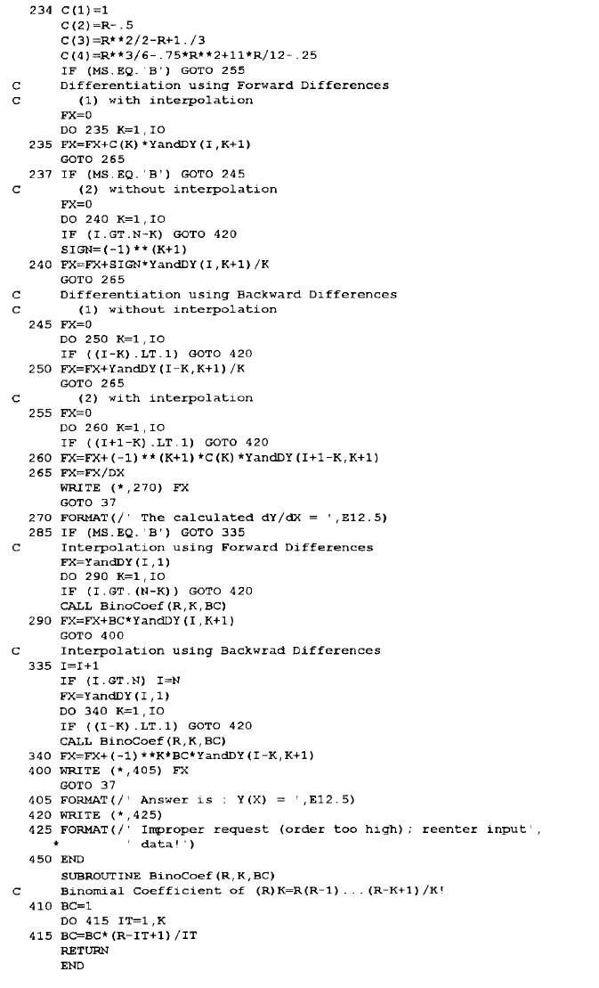
FORTRAN VERSION