Munson B.R. Fundamentals of Fluid Mechanics

Подождите немного. Документ загружается.

187

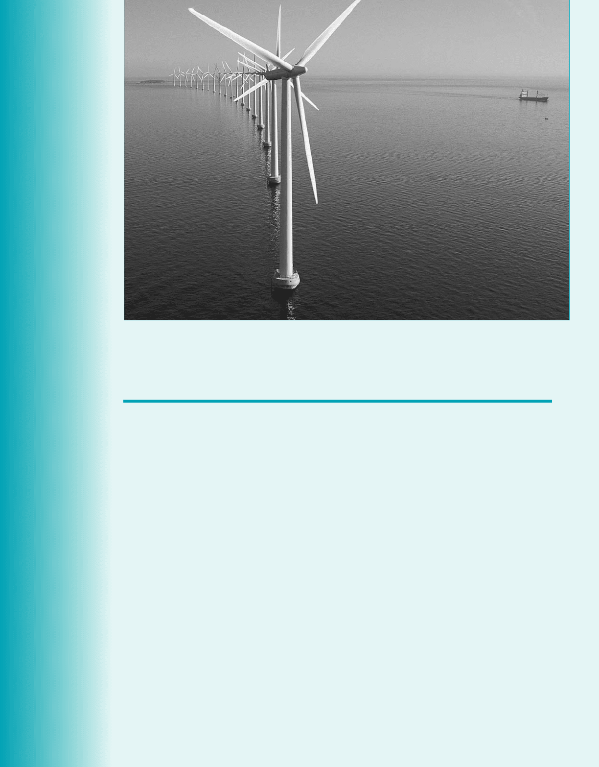
CHAPTER OPENING PHOTO: Wind turbine farms (this is the Middelgrunden Offshore Wind Farm in Denmark)

are becoming more common. Finite control volume analysis can be used to estimate the amount of energy

transferred between the moving air and each turbine rotor. (Photograph courtesy of Siemens Wind Power.)

Learning Objectives

After completing this chapter, you should be able to:

■ select an appropriate finite control volume to solve a fluid mechanics problem.

■ apply conservation of mass and energy and Newton’s second law of motion to

the contents of a finite control volume to get important answers.

■ know how velocity changes and energy transfers in fluid flows are related to

forces and torques.

■ understand why designing for minimum loss of energy in fluid flows is so

important.

To solve many practical problems in fluid mechanics, questions about the behavior of the contents

of a finite region in space 1a finite control volume2are answered. For example, we may be asked

to estimate the maximum anchoring force required to hold a turbojet engine stationary during a

test. Or we may be called on to design a propeller to move a boat both forward and backward. Or

we may need to determine how much power it would take to move natural gas from one location

to another many miles away.

The bases of finite control volume analysis are some fundamental laws of physics, namely,

conservation of mass, Newton’s second law of motion, and the first and second laws of thermody-

namics. While some simplifying approximations are made for practicality, the engineering answers

possible with the estimates of this powerful analysis method have proven valuable in numerous in-

stances.

Conservation of mass is the key to tracking flowing fluid. How much enters and leaves a

control volume can be ascertained.

inite Control

Volume Analysis

inite Control

Volume Analysis

Many fluid me-

chanics problems

can be solved by us-

ing control volume

analysis.

JWCL068_ch05_187-262.qxd 9/23/08 9:53 AM Page 187

Newton’s second law of motion leads to the conclusion that forces can result from or cause

changes in a flowing fluid’s velocity magnitude and/or direction. Moment of force 1torque2can re-

sult from or cause changes in a flowing fluid’s moment of velocity. These forces and torques can

be associated with work and power transfer.

The first law of thermodynamics is a statement of conservation of energy. The second law

of thermodynamics identifies the loss of energy associated with every actual process. The me-

chanical energy equation based on these two laws can be used to analyze a large variety of steady,

incompressible flows in terms of changes in pressure, elevation, speed, and of shaft work and loss.

Good judgment is required in defining the finite region in space, the control volume, used

in solving a problem. What exactly to leave out of and what to leave in the control volume are im-

portant considerations. The formulas resulting from applying the fundamental laws to the contents

of the control volume are easy to interpret physically and are not difficult to derive and use.

Because a finite region of space, a control volume, contains many fluid particles and even

more molecules that make up each particle, the fluid properties and characteristics are often aver-

age values. In Chapter 6 an analysis of fluid flow based on what is happening to the contents of

an infinitesimally small region of space or control volume through which numerous molecules

simultaneously flow (what we might call a point in space) is considered.

188 Chapter 5 ■ Finite Control Volume Analysis

5.1.1 Derivation of the Continuity Equation

A system is defined as a collection of unchanging contents, so the conservation of mass principle

for a system is simply stated as

time rate of change of the system mass

(5.1)

where the system mass, is more generally expressed as

(5.2)

and the integration is over the volume of the system. In words, Eq. 5.2 states that the system mass

is equal to the sum of all the density-volume element products for the contents of the system.

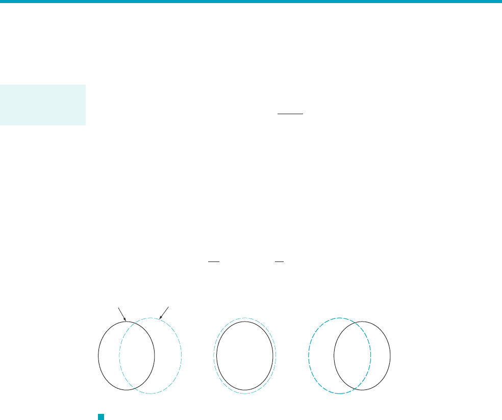
For a system and a fixed, nondeforming control volume that are coincident at an instant of

time, as illustrated in Fig. 5.1, the Reynolds transport theorem 1Eq. 4.192with and

allows us to state that

(5.3)

冮

sys

r dV⫺⫽

冮

r dV⫺⫹

冮

rV ⴢ nˆ dA

b ⫽ 1B ⫽ mass

sys

⫽

冮

sys

r dV⫺

sys

⫽ 0

5.1 Conservation of Mass—The Continuity Equation

The amount of

mass in a system is

constant.

System

Control Volume

(

a)(b

)(

F I G U R E 5.1 System and control volume at three different

instances of time. (a) System and control volume at time . (b) System and

control volume at time t, coincident condition. (c) System and control volume at

time .t ⴙ Dt

t ⴚ Dt

JWCL068_ch05_187-262.qxd 9/23/08 9:53 AM Page 188

In Eq. 5.3, we express the time rate of change of the system mass as the sum of two control vol-

ume quantities, the time rate of change of the mass of the contents of the control volume,

and the net rate of mass flow through the control surface,

When a flow is steady, all field properties 1i.e., properties at any specified point2including

density remain constant with time and the time rate of change of the mass of the contents of the

control volume is zero. That is,

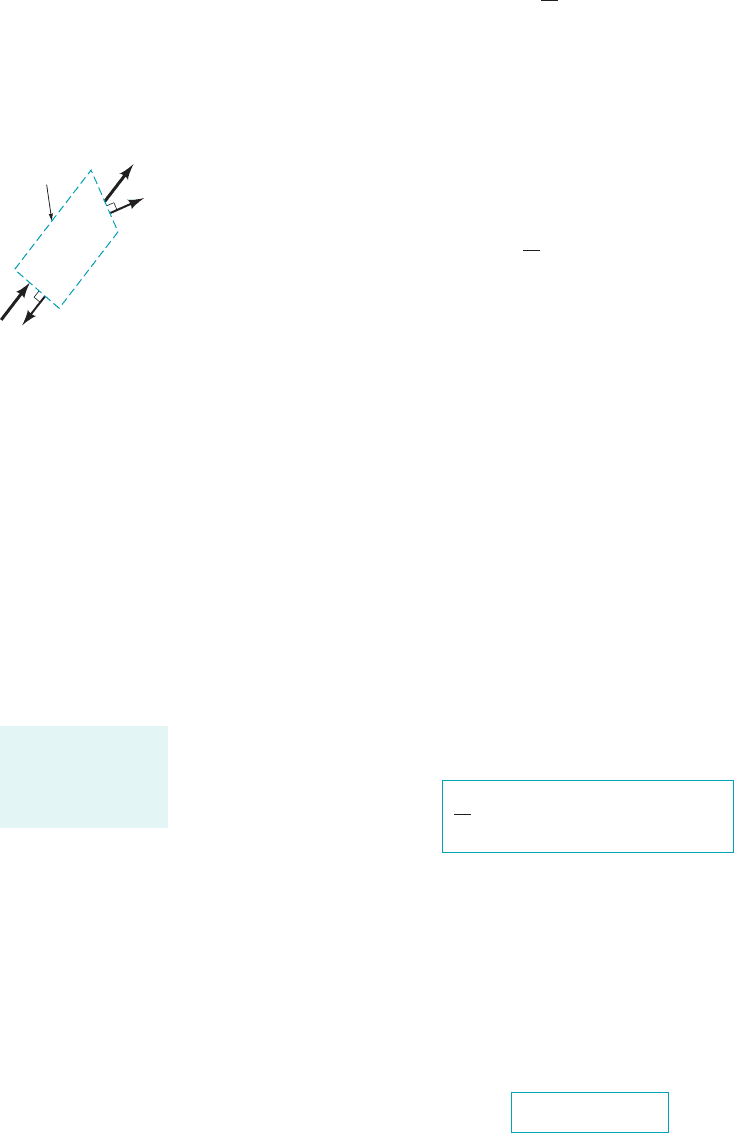
The integrand, in the mass flowrate integral represents the product of the compo-

nent of velocity, V, perpendicular to the small portion of control surface and the differential area,

dA. Thus, is the volume flowrate through dA and is the mass flowrate through

dA. Furthermore, as shown in the sketch in the margin, the sign of the dot product is

for flow out of the control volume and for flow into the control volume since is considered

positive when it points out of the control volume. When all of the differential quantities,

are summed over the entire control surface, as indicated by the integral

the result is the net mass flowrate through the control surface, or

(5.4)

where is the mass flowrate If the integral in Eq. 5.4 is positive, the net flow

is out of the control volume; if the integral is negative, the net flow is into the control volume.

The control volume expression for conservation of mass, which is commonly called the con-

tinuity equation, for a fixed, nondeforming control volume is obtained by combining Eqs. 5.1, 5.2,

and 5.3 to obtain

(5.5)

In words, Eq. 5.5 states that to conserve mass the time rate of change of the mass of the contents

of the control volume plus the net rate of mass flow through the control surface must equal zero.

Actually, the same result could have been obtained more directly by equating the rates of mass flow

into and out of the control volume to the rates of accumulation and depletion of mass within the

control volume 1see Section 3.6.22. It is reassuring, however, to see that the Reynolds transport the-

orem works for this simple-to-understand case. This confidence will serve us well as we develop

control volume expressions for other important principles.

An often-used expression for mass flowrate, through a section of control surface having

area A is

(5.6)m

⫽ rQ ⫽ rAV

冮

r dV⫺⫹

冮

rV ⴢ nˆ dA ⫽ 0

1lbm

Ⲑ

s, slug

Ⲑ

s or kg

Ⲑ

s2.m

冮

rV ⴢ nˆ dA ⫽

out

⫺

冮

rV ⴢ nˆ dA

rV ⴢ nˆ dA,

nˆ“⫺”

“⫹”V ⴢ nˆ

rV ⴢ nˆ dAV ⴢ nˆ dA

V ⴢ nˆ dA,

冮

r dV⫺⫽0

冮

rV ⴢ nˆ dA

冮

r dV⫺

time rate of change

of the mass of the

coincident system

⫽

time rate of change

of the mass of the

contents of the coin-

cident control volume

⫹

net rate of flow

of mass through

the control

surface

5.1 Conservation of Mass—The Continuity Equation 189

Control

surface

V⭈n > 0

V⭈n < 0

The continuity

equation is a state-

ment that mass is

conserved.

JWCL068_ch05_187-262.qxd 9/23/08 9:53 AM Page 189

where is the fluid density, Q is the volume flowrate and V is the component of

fluid velocity perpendicular to area A. Since

application of Eq. 5.6 involves the use of representative or average values of fluid density, and

fluid velocity, V. For incompressible flows, is uniformly distributed over area A. For compress-

ible flows, we will normally consider a uniformly distributed fluid density at each section of flow

and allow density changes to occur only from section to section. The appropriate fluid velocity to

use in Eq. 5.6 is the average value of the component of velocity normal to the section area in-

volved. This average value, defined as

(5.7)

is shown in the figure in the margin.

If the velocity is considered uniformly distributed 1one-dimensional flow2over the section

area, A, then

(5.8)

and the bar notation is not necessary 1as in Example 5.12. When the flow is not uniformly distrib-

uted over the flow cross-sectional area, the bar notation reminds us that an average velocity is be-

ing used 1as in Examples 5.2 and 5.42.

5.1.2 Fixed, Nondeforming Control Volume

In many applications of fluid mechanics, an appropriate control volume to use is fixed and nonde-

forming. Several example problems that involve the continuity equation for fixed, nondeforming

control volumes 1Eq. 5.52follow.

⫽

冮

rV ⴢ nˆ dA

⫽ V

V ⫽

冮

rV ⴢ nˆ dA

⫽

冮

rV ⴢ nˆ dA

1ft

Ⲑ

s or m

Ⲑ

s2,r

190 Chapter 5 ■ Finite Control Volume Analysis

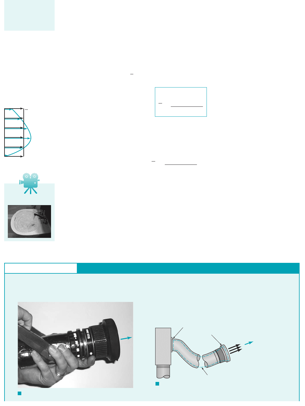
V5.1 Sink flow

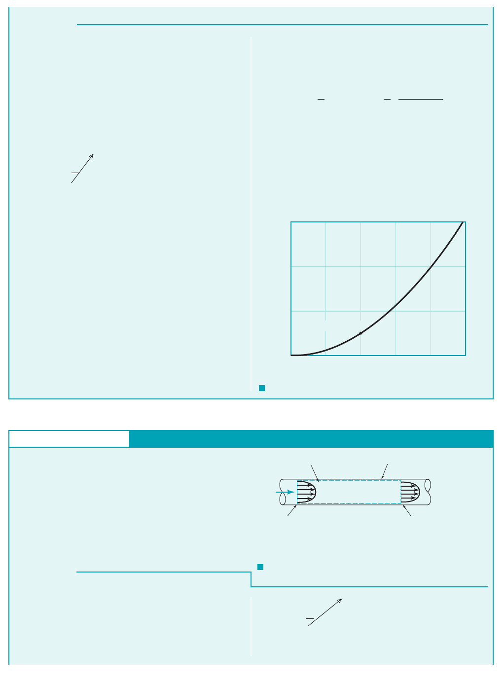
GIVEN Water flows steadily through a nozzle at the end of a

fire hose as illustrated in Fig. E5.1a. According to local regula-

tions, the nozzle exit velocity must be at least 20 m/s as shown in

Fig. E5.1b.

FIND Determine the minimum pumping capacity, Q, required

in m

/s.

F I G U R E E5.1

Conservation of Mass—Steady, Incompressible Flow

Section (1) (pump discharge)

Flow

Control volume

= 20 m/s

= 40 mm

Section (2) (nozzle exit)

XAMPLE 5.1

Mass flowrate

equals the product

of density and vol-

ume flowrate.

JWCL068_ch05_187-262.qxd 9/23/08 9:53 AM Page 190

5.1 Conservation of Mass—The Continuity Equation 191

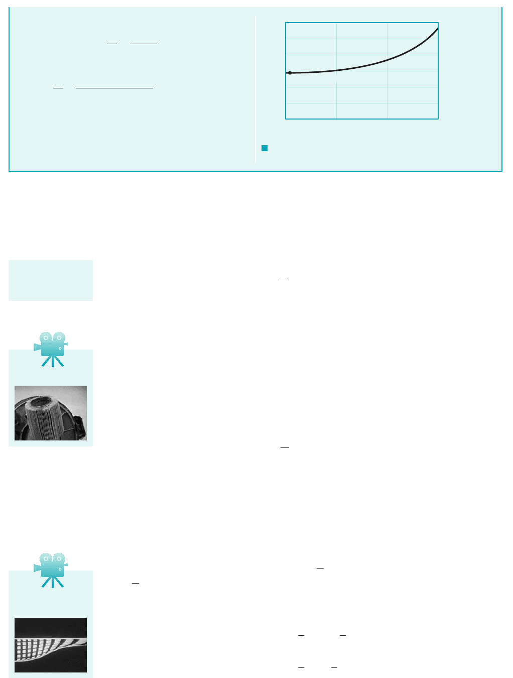
The pumping capacity is equal to the volume flowrate at the nozzle

exit. If, for simplicity, the velocity distribution at the nozzle exit plane,

section (2), is considered uniform (one-dimensional), then from Eq. 5

(Ans)

COMMENT By repeating the calculations for various val-

ues of the nozzle exit diameter, D

, the results shown in Fig.

E5.1c are obtained. The flowrate is proportional to the exit area,

which varies as the diameter squared. Hence, if the diameter

were doubled, the flowrate would increase by a factor of four,

provided the exit velocity remained the same.

⫽ 0.0251 m

⫽ V

␲

⫽ 120 m/s2

␲

40 mm

1000 mm/m

⫽ Q

⫽ V

F I G U R E E5.1

0.15

0.10

0.05

0 20 40 60 80 100

, mm

(40 mm, 0.0251 m

/s)

OLUTION

The pumping capacity sought is the volume flowrate delivered by

the fire pump to the hose and nozzle. Since we desire knowledge

about the pump discharge flowrate and we have information

about the nozzle exit flowrate, we link these two flowrates with

the control volume designated with the dashed line in Fig. E5.1b.

This control volume contains, at any instant, water that is within

the hose and nozzle from the pump discharge to the nozzle exit

plane.

Equation 5.5 is applied to the contents of this control volume

to give

0 (flow is steady)

(1)

The time rate of change of the mass of the contents of this control

volume is zero because the flow is steady. Because there is only

one inflow [the pump discharge, section (1)] and one outflow [the

nozzle exit, section (2)], Eq. (1) becomes

so that with

(2)

Because the mass flowrate is equal to the product of fluid density, ␳,

and volume flowrate, Q (see Eq. 5.6), we obtain from Eq. 2

(3)

Liquid flow at low speeds, as in this example, may be considered

incompressible. Therefore

(4)

and from Eqs. 3 and 4

(5)Q

⫽ Q

␳

⫽ ␳

␳

⫽ ␳

⫽ m

⫽ ␳AV

␳

⫺ ␳

⫽ 0

冮

r dV⫺⫹

冮

rV ⴢ n

dA ⫽ 0

GIVEN Air flows steadily between two sections in a long,

straight portion of 4-in. inside diameter pipe as indicated in

Fig. E5.2. The uniformly distributed temperature and pressure at

each section are given. The average air velocity 1nonuniform ve-

locity distribution2at section 122is

FIND Calculate the average air velocity at section 112.

1000 ft

Ⲑ

OLUTION

F I G U R E E5.2

Conservation of Mass—Steady, Compressible Flow

Control volume

Flow

Section (1)

= 100 psia

= 540 °R

= 18.4 psia

= 453 °R

= 1000 ft/s

= D

= 4 in.

Section (2)

Pipe

XAMPLE 5.2

The average fluid velocity at any section is that velocity which

yields the section mass flowrate when multiplied by the section

average fluid density and section area 1Eq. 5.72. We relate the

flows at sections 112and 122with the control volume designated

with a dashed line in Fig. E5.2.

Equation 5.5 is applied to the contents of this control volume

to obtain

0 1flow is steady2

The time rate of change of the mass of the contents of this control

volume is zero because the flow is steady. The control surface

冮

r dV⫺⫹

冮

rV ⴢ nˆ dA ⫽ 0

JWCL068_ch05_187-262.qxd 9/23/08 9:53 AM Page 191

192 Chapter 5 ■ Finite Control Volume Analysis

integral involves mass flowrates at sections 112and 122so that from

Eq. 5.4 we get

(1)

and from Eqs. 1, 5.6, and 5.7 we obtain

(2)

or since

(3)

Air at the pressures and temperatures involved in this example

problem behaves like an ideal gas. The ideal gas equation of state

1Eq. 1.82is

(4)r ⫽

⫽

⫽ A

⫽ r

⫽ m

冮

rV ⴢ nˆ dA ⫽ m

⫺ m

⫽ 0

Thus, combining Eqs. 3 and 4 we obtain

(Ans)

COMMENT We learn from this example that the continuity

equation 1Eq. 5.52is valid for compressible as well as incom-

pressible flows. Also, nonuniform velocity distributions can be

handled with the average velocity concept. Significant average ve-

locity changes can occur in pipe flow if the fluid is compressible.

⫽

118.4 psia21540 °R211000 ft

Ⲑ

1100 psia21453 °R2

⫽ 219 ft

Ⲑ

⫽

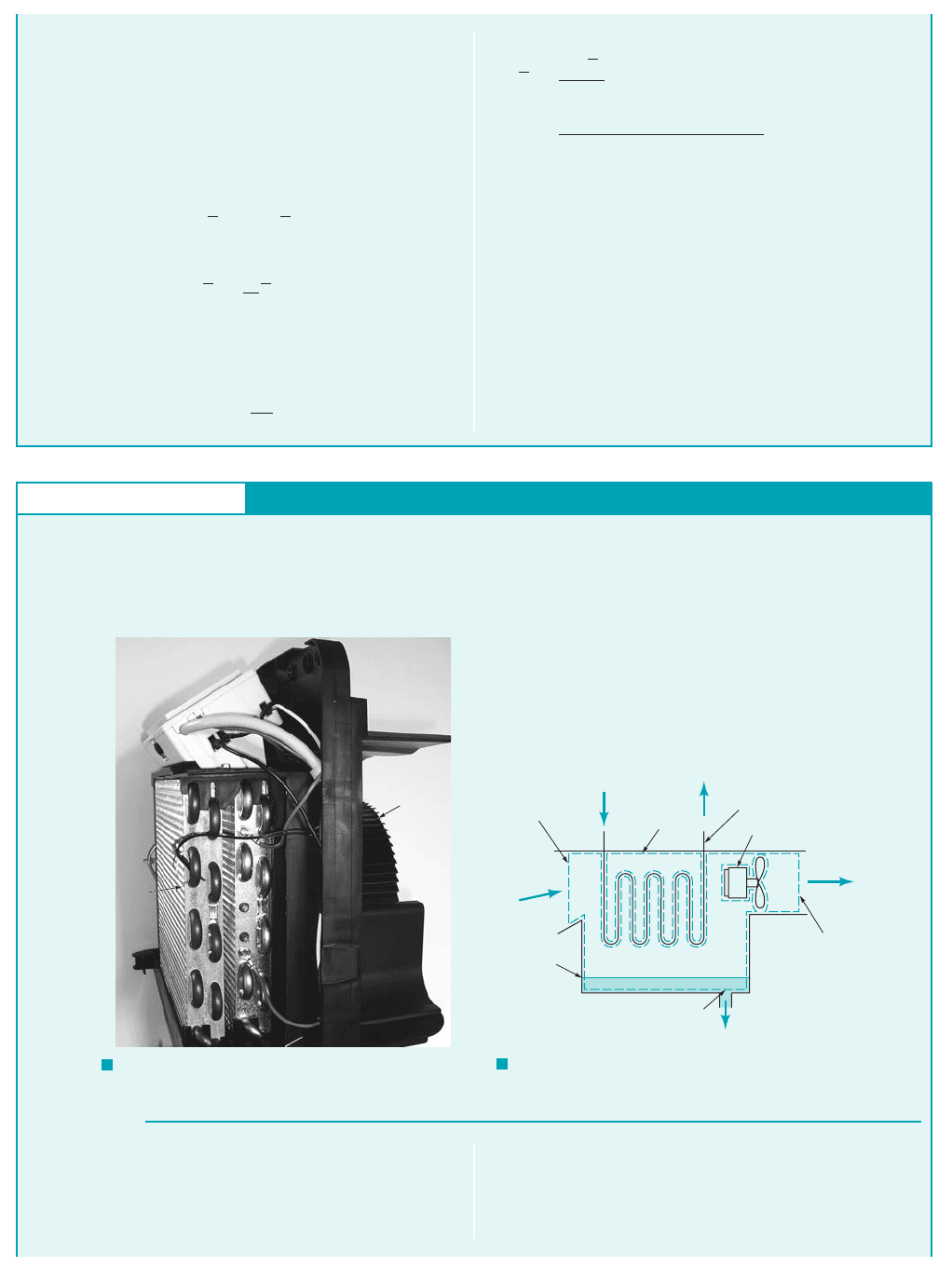
GIVEN The inner workings of a dehumidifier are shown in

Fig. E5.3a. Moist air 1a mixture of dry air and water vapor2enters

the dehumidifier at the rate of 600 lbm兾hr. Liquid water drains out

of the dehumidifier at a rate of 3.0 lbm兾hr. A simplified sketch of

the process is provided in Fig. E5.3b.

FIND Determine the mass flowrate of the dry air and the water

vapor leaving the dehumidifier.

F I G U R E E5.3

Conservation of Mass—Two Fluids

Cooling

coil

Fan

F I G U R E E5.3

Fan

Motor

Cooling coil

Control volume

Condensate

(water)

Section (1)

Section (3)

Section (2)

•

600 lbm/hr

•

= 3.0 lbm/hr

•

= ?

•

XAMPLE 5.3

Not included in the control volume are the fan and its motor,

and the condenser coils and refrigerant. Even though the flow in

the vicinity of the fan blade is unsteady, it is unsteady in a cycli-

cal way. Thus, the flowrates at sections 112, 122, and 132appear

steady and the time rate of change of the mass of the contents of

OLUTION

The unknown mass flowrate at section 122is linked with the known

flowrates at sections 112and 132with the control volume designated

with a dashed line in Fig. E5.3b. The contents of the control vol-

ume are the air and water vapor mixture and the condensate 1liq-

uid water2in the dehumidifier at any instant.

JWCL068_ch05_187-262.qxd 9/23/08 9:54 AM Page 192

5.1 Conservation of Mass—The Continuity Equation 193

the control volume may be considered equal to zero on a time-

average basis. The application of Eqs. 5.4 and 5.5 to the control

volume contents results in

(Ans)

COMMENT Note that the continuity equation 1Eq. 5.52can

be used when there is more than one stream of fluid flowing

through the control volume.

⫽ 597 lbm

Ⲑ

⫽ m

⫺ m

⫽ 600 lbm

Ⲑ

hr ⫺ 3.0 lbm

Ⲑ

冮

rV ⴢ nˆ dA ⫽⫺m

⫹ m

⫽ 0

The answer is the same with a control volume which includes

the cooling coils to be within the control volume. The continuity

equation becomes

(1)

where is the mass flowrate of the cooling fluid flowing

into the control volume, and is the flowrate out of the

control volume through the cooling coil. Since the flow

through the coils is steady, it follows that . Hence,

Eq. 1 gives the same answer as obtained with the original con-

trol volume.

⫽ m

⫺ m

⫹ m

⫺ m

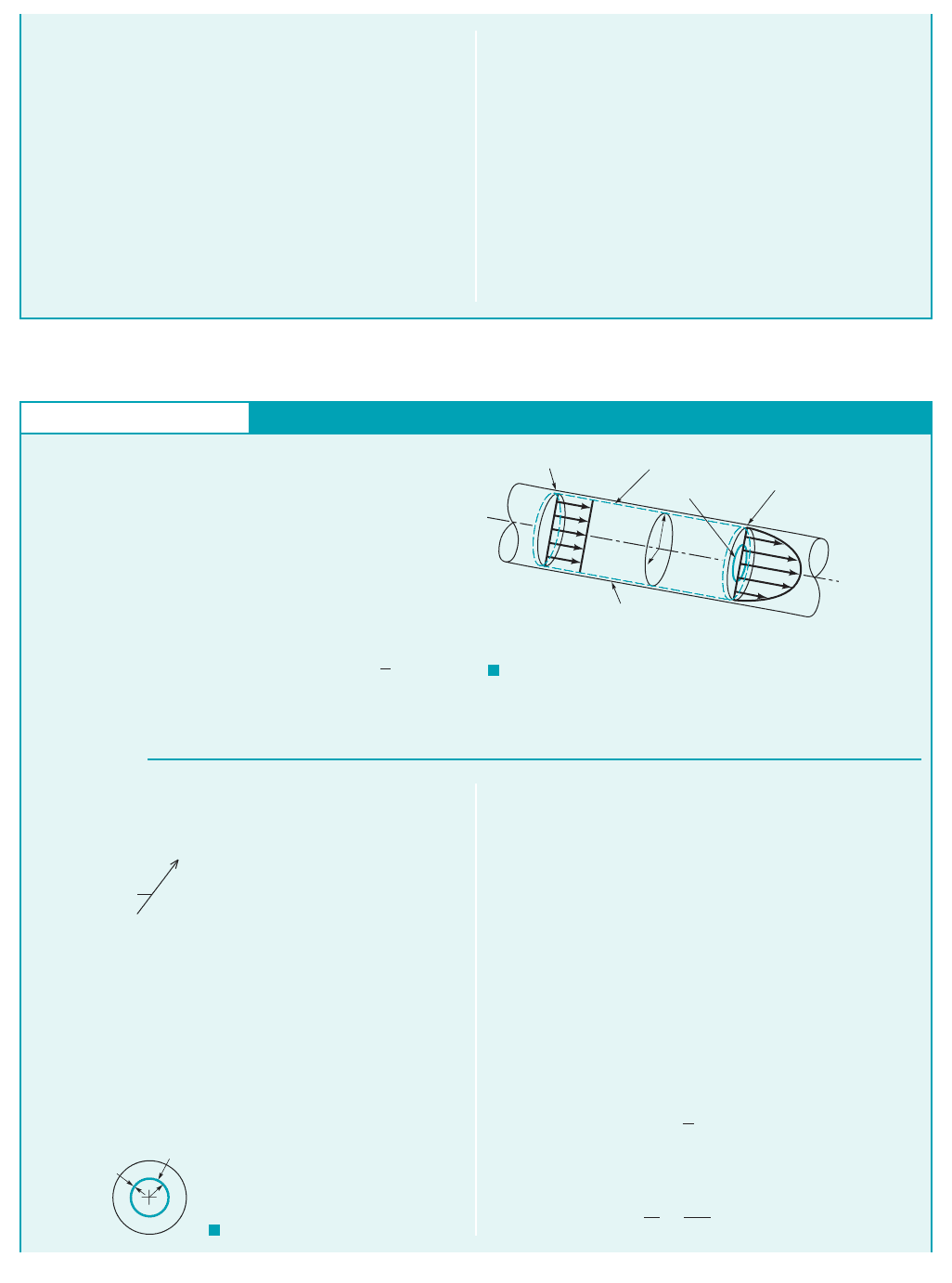
GIVEN Incompressible, laminar water flow develops in a

straight pipe having radius R as indicated in Fig. E5.4a. At section

(1), the velocity profile is uniform; the velocity is equal to a con-

stant value U and is parallel to the pipe axis everywhere. At sec-

tion (2), the velocity profile is axisymmetric and parabolic, with

zero velocity at the pipe wall and a maximum value of u

max

at the

centerline.

FIND

(a) How are U and u

max

related?

(b) How are the average velocity at section (2), , and u

max

related?

OLUTION

F I G U R E E5.4

Conservation of Mass—Nonuniform Velocity Profile

Section (1) Control volume

= 2 r dr

Section (2)

Pipe

= U

= u

max

1 -

( )

[ ]

XAMPLE 5.4

(a) An appropriate control volume is sketched (dashed lines) in

Fig. E5.4a. The application of Eq. 5.5 to the contents of this con-

trol volume yields

0 (flow is steady)

(1)

At the inlet, section (1), the velocity is uniform with V

⫽ U so

that

(2)

At the outlet, section (2), the velocity is not uniform. How-

ever, the net flowrate through this section is the sum of flows

through numerous small washer-shaped areas of size dA

⫽ 2␲r dr

as shown by the shaded area element in Fig. E5.4b. On each of

冮

112

rV ⴢ

n dA ⫽⫺r

冮

r dV⫺⫹

冮

rV ⴢ n

dA ⫽ 0

F I G U R E E5.4

these infinitesimal areas the fluid velocity is denoted as u

Thus, in the limit of infinitesimal area elements, the summation

is replaced by an integration and the outflow through section (2)

is given by

(3)

By combining Eqs. 1, 2, and 3 we get

(4)

Since the flow is considered incompressible, ␳

⫽ ␳

. The para-

bolic velocity relationship for flow through section (2) is used in

Eq. 4 to yield

(5)

Integrating, we get from Eq. 5

2␲u

max

⫺

⫺ ␲R

U ⫽ 0

2␲u

max

冮

c1 ⫺ a

dr dr ⫺ A

U ⫽ 0

␳

冮

2␲r dr ⫺ ␳

U ⫽ 0

冮

122

rV ⴢ

n dA ⫽ r

冮

2pr dr

JWCL068_ch05_187-262.qxd 9/23/08 9:54 AM Page 193

194 Chapter 5 ■ Finite Control Volume Analysis

(Ans)

(b) Since this flow is incompressible, we conclude from Eq.

5.7 that U is the average velocity at all sections of the control vol-

ume. Thus, the average velocity at section (2), , is one-half the

maximum velocity, u

max

, there or

(Ans)

COMMENT The relationship between the maximum veloc-

ity at section (2) and the average velocity is a function of the

“shape” of the velocity profile. For the parabolic profile as-

sumed in this example, the average velocity, is the actual

“average” of the maximum velocity at section (2),

and the minimum velocity at that section, u

⫽ 0. However, as

shown in Fig. E5.4c, if the velocity profile is a different shape

(non-parabolic), the average velocity is not necessarily one half

of the maximum velocity.

⫽ u

max

/2,

⫽

max

⫽ 2U

= u

max

(parabolic)

= u

max

(non-parabolic)

max

F I G U R E E5.4

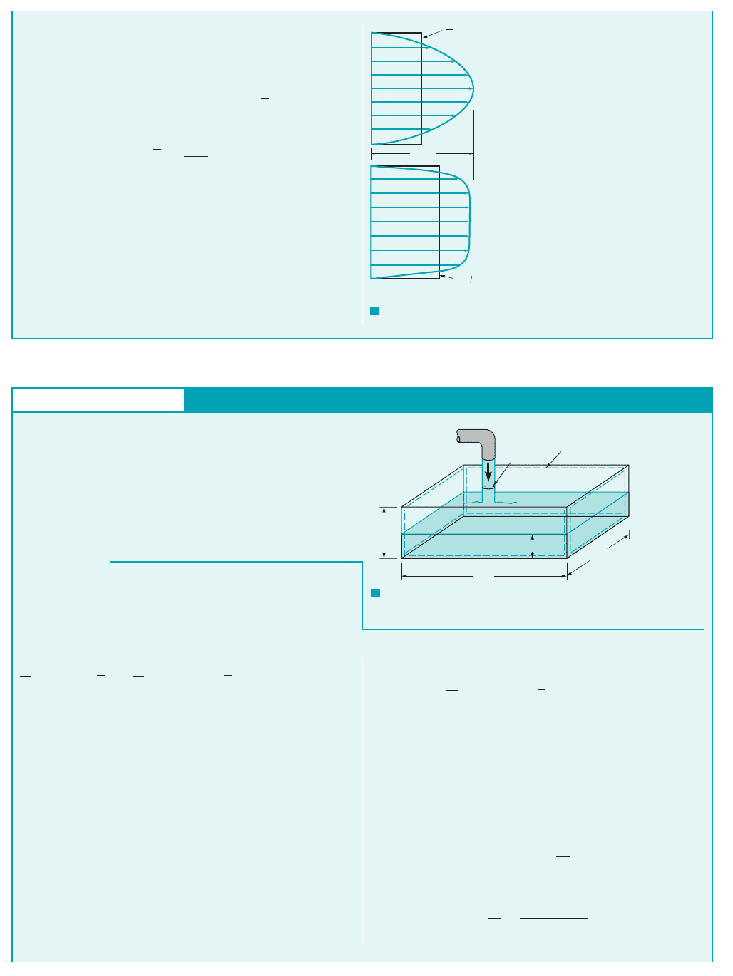
GIVEN A bathtub is being filled with water from a faucet. The

rate of flow from the faucet is steady at 9 gal/min. The tub volume

is approximated by a rectangular space as indicated in Fig. E5.5a.

FIND Estimate the time rate of change of the depth of water in

the tub, ∂h/∂t, in inches per minute at any instant.

OLUTION

F I G U R E E5.5

Conservation of Mass—Unsteady Flow

for air, and

(2)

for water. The volume of water in the control volume is given by

(3)

where A

is the cross-sectional area of the water flowing from the

faucet into the tub. Combining Eqs. 2 and 3, we obtain

and, thus, since

⫽

water

110 ft

⫺ A

⫽ ␳Q,

␳

water

110 ft

⫺ A

⫽ m

water

⫹ 11.5 ft ⫺ h2A

冮

water

volume

␳

water

⫽ ␳

water

3h12 ft215 ft2

冮

water

volume

␳

water

⫽ m

water

2 ft

5 ft

1.5 ft

Control volume

XAMPLE 5.5

We use the fixed, nondeforming control volume outlined with a

dashed line in Fig. E5.5a. This control volume includes in it, at

any instant, the water accumulated in the tub, some of the water

flowing from the faucet into the tub, and some air. Application of

Eqs. 5.4 and 5.5 to these contents of the control volume results in

(1)

Recall that the mass, dm, of fluid contained in a small volume

is . Hence, the two integrals in Eq. 1 represent the

total amount of air and water in the control volume, and the sum

of the first two terms is the time rate of change of mass within

the control volume.

Note that the time rate of change of air mass and water mass

are each not zero. Recognizing, however, that the air mass must

be conserved, we know that the time rate of change of the mass of

air in the control volume must be equal to the rate of air mass flow

out of the control volume. For simplicity, we disregard any water

evaporation that occurs. Thus, applying Eqs. 5.4 and 5.5 to the air

only and to the water only, we obtain

冮

air

volume

␳

air

⫹ m

air

⫽ 0

dm ⫽ ␳ dV

⫺ m

water

⫹ m

air

⫽ 0

冮

air

volume

␳

air

⫹

冮

water

volume

␳

water

JWCL068_ch05_187-262.qxd 9/23/08 9:54 AM Page 194

The preceding example problems illustrate some important results of applying the conserva-

tion of mass principle to the contents of a fixed, nondeforming control volume. The dot product

is for flow out of the control volume and for flow into the control volume. Thus,

mass flowrate out of the control volume is and mass flowrate in is When the flow is

steady, the time rate of change of the mass of the contents of the control volume

is zero and the net amount of mass flowrate, through the control surface is therefore also zero

(5.9)

If the steady flow is also incompressible, the net amount of volume flowrate, Q, through the con-

trol surface is also zero:

(5.10)

An unsteady, but cyclical flow can be considered steady on a time-average basis. When the flow

is unsteady, the instantaneous time rate of change of the mass of the contents of the control vol-

ume is not necessarily zero and can be an important variable. When the value of

is the mass of the contents of the control volume is increasing. When it is the mass of

the contents of the control volume is decreasing.

When the flow is uniformly distributed over the opening in the control surface 1one-dimensional

flow2,

where V is the uniform value of the velocity component normal to the section area A. When the

velocity is nonuniformly distributed over the opening in the control surface,

(5.11)

where is the average value of the component of velocity normal to the section area A as defined

by Eq. 5.7.

For steady flow involving only one stream of a specific fluid flowing through the control vol-

ume at sections 112and 122,

(5.12)

and for incompressible flow,

(5.13)Q  A

 A

 r

 rAV

“,”“,”

冮

r dV

out



 0

out



 0

冮

r dV

“.”“”

“”“”V ⴢ nˆ

5.1 Conservation of Mass—The Continuity Equation 195

For A

 10 ft

we can conclude that

(Ans)

COMMENT By repeating the calculations for the same

flowrate but with various water jet diameters, D

, the results

shown in Fig. E5.5bare obtained. With the flowrate held constant,

the value of is nearly independent of the jet diameter for val-

ues of the diameter less than about 10 in.

0h/0t



19 gal/min2112 in./ft2

17.48 gal/ft

2110 ft

 1.44 in./min



water

110 ft

2.5

1.5

0.5

0 10 20 30

∂h/∂t, in./min

(1 in., 1.44 in./min)

, in.

F I G U R E E5.5

The appropriate

sign convention

must be followed.

V5.2 Shop vac filter

V5.3 Flow through

a contraction

JWCL068_ch05_187-262.qxd 9/23/08 9:54 AM Page 195

For steady flow involving more than one stream of a specific fluid or more than one specific

fluid flowing through the control volume,

The variety of example problems solved above should give the correct impression that the

fixed, nondeforming control volume is versatile and useful.

⫽

out

196 Chapter 5 ■ Finite Control Volume Analysis

Fluids in the News

New 1.6 GPF standards Toilets account for approximately 40%

of all indoor household water use. To conserve water, the new

standard is 1.6 gallons of water per flush (gpf). Old toilets use

up to 7 gpf; those manufactured after 1980 use 3.5 gpf. Neither

are considered low-flush toilets. A typical 3.2 person household

in which each person flushes a 7-gpf toilet 4 times a day uses

32,700 gallons of water each year; with a 3.5-gpf toilet the

amount is reduced to 16,400 gallons. Clearly the new 1.6-gpf

toilets will save even more water. However, designing a toilet

that flushes properly with such a small amount of water is not

simple. Today there are two basic types involved: those that are

gravity powered and those that are pressure powered. Gravity

toilets (typical of most currently in use) have rather long cycle

times. The water starts flowing under the action of gravity and the

swirling vortex motion initiates the siphon action which builds to

a point of discharge. In the newer pressure-assisted models, the

flowrate is large but the cycle time is short and the amount of

water used is relatively small. (See Problem 5.32.)

5.1.3 Moving, Nondeforming Control Volume

It is sometimes necessary to use a nondeforming control volume attached to a moving reference

frame. Examples include control volumes containing a gas turbine engine on an aircraft in flight,

the exhaust stack of a ship at sea, and the gasoline tank of an automobile passing by.

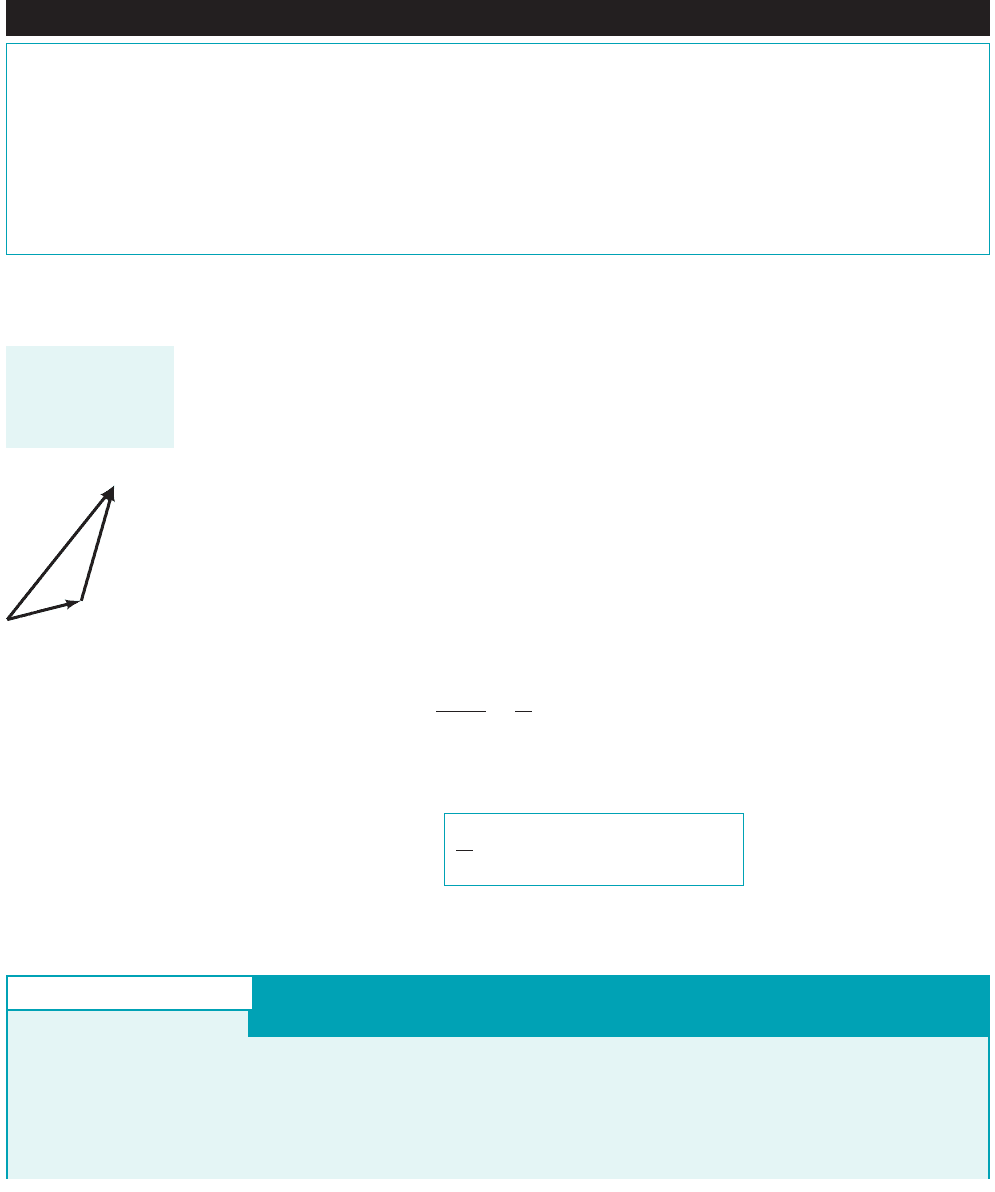
As discussed in Section 4.4.6, when a moving control volume is used, the fluid velocity rela-

tive to the moving control volume 1relative velocity2is an important flow field variable. The relative

velocity, W, is the fluid velocity seen by an observer moving with the control volume. The control

volume velocity, is the velocity of the control volume as seen from a fixed coordinate system.

The absolute velocity, V, is the fluid velocity seen by a stationary observer in a fixed coordinate sys-

tem. These velocities are related to each other by the vector equation

(5.14)

as illustrated by the figure in the margin. This is the same as Eq. 4.22, introduced earlier.

For a system and a moving, nondeforming control volume that are coincident at an instant

of time, the Reynolds transport theorem 1Eq. 4.232for a moving control volume leads to

(5.15)

From Eqs. 5.1 and 5.15, we can get the control volume expression for conservation of mass

1the continuity equation2for a moving, nondeforming control volume, namely,

(5.16)

Some examples of the application of Eq. 5.16 follow.

冮

r dV⫺⫹

冮

rW ⴢ nˆ dA ⫽ 0

sys

⫽

冮

r dV⫺⫹

冮

rW ⴢ nˆ dA

V ⫽ W ⫹ V

Some problems are

most easily solved

by using a moving

control volume.

GIVEN An airplane moves forward at a speed of as

shown in Fig. E5.6a. The frontal intake area of the jet engine is

and the entering air density is A stationary

observer determines that relative to the earth, the jet engine

exhaust gases move away from the engine with a speed of

0.736 kg

Ⲑ

0.80 m

971 km

Ⲑ

Conservation of Mass—Compressible Flow with

a Moving Control Volume

The engine exhaust area is , and the exhaust

gas density is

FIND Estimate the mass flowrate of fuel into the engine in

Ⲑ

hr.

0.515 kg

Ⲑ

0.558 m

1050 km

Ⲑ

hr.

XAMPLE 5.6

JWCL068_ch05_187-262.qxd 9/23/08 9:54 AM Page 196