Menke W. Geophysical Data Analysis: Discrete Inverse Theory

Подождите немного. Документ загружается.

178

Continuous

Inverse

Theory

and

Tomography

In realistic experiments,

d(u,8)

is sampled only at discrete points

d(ui,Oi).

Nevertheless, much insight can be gained into the behavior of

Eq.

1.19) by regarding

(u,8)

as continuous variables. Equation

(

1.19) is then an integral transform that transforms variables

(x,y)

two new variables

(u,8)

and is called a Radon transform.

11.6

The Fourier Slice Theorem

The Radon transform is similar to another integral transform, the

Fourier transform, which transforms spatial position

to spatial wave

number

k,:

f(kJ

rf(x)

exp(ik,x)

and

f(x)

_f_

/+-mflk,)

exp(-

ik,x)

1.20)

--a0

In fact, the two are quite closely related, as can

seen by Fourier

transforming Eq.

1.19) with respect to

k,:

&k,,8)

1.;

m(x

cos

sin

--m

sin

cos

exp(ik,u)

1.21)

We now transform the double integral from

ds du

dx dy,

using the

fact that the Jacobian determinant

ld(x,y)/a(u,s)l

is unity [see

Eq.

(1 1.18)]

/+-

I-;

m(x,y)

exp(ik, cos

ik, sin

du ds

-m

&(k,

cos

sin

.22)

This result, called the Fourier slice theorem, provides a method of

inverting the Radon transform. The Fourier-tra;sformed quantity

&k,

$3)

simply the Fourier-transformed image

&(k,,k,)

evaluated

along radial lines in the

(k,,k,)

plane (Fig. 11.3). If the Radon trans-

form is known for all values of

(u,8),

then the Fourier-transformed

image is known for all

(k,,k,).

The space domain image

m(x,y)

found by taking the inverse Fourier transform.

1 1.7

Backprojection

179

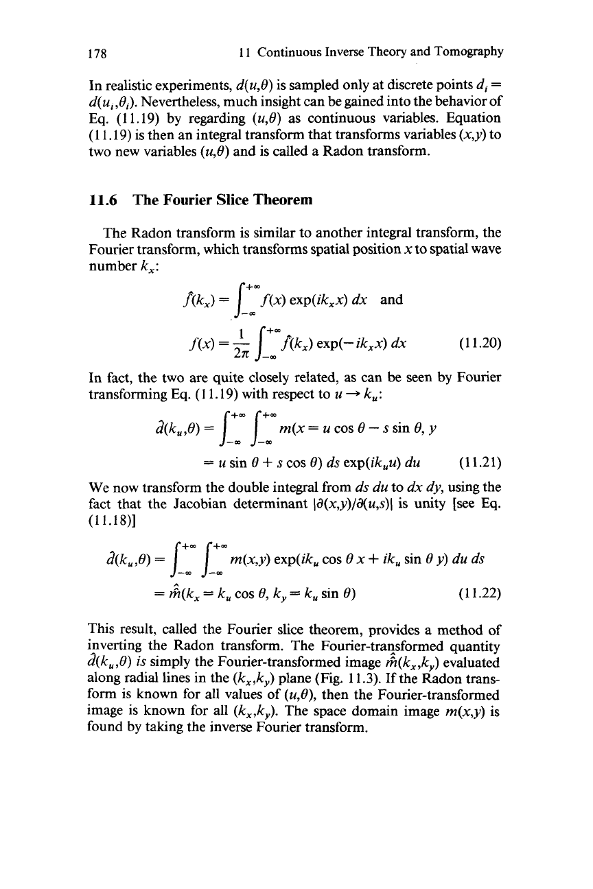
Fig.

11.3.

(Left)

The function

m(x,y)

is integrated along a set of parallel lines (dashed) in

a Radon transform to form the function

d(u,O,).

This function is called the projection of

at angle

0,.

(Right)

The Fourier slice theorem states that the Fourier transform of the

projection (here denoted

is equal to te Fourier-transformed image

A(k,,k,)

evalu-

ated along a line (bold) in the

(k,,k,)

plane.

Since the Fourier transform and its inverse are unique, the Radon

transform can

uniquely inverted if it is known for all possible

(u,8).

Furthermore, the Fourier slice theorem can

used to invert the

Radon transform in practice by using discrete Fourier transforms in

place of integral Fourier transforms. However,

must

sampled

sufficiently evenly that the

transcorm can be performed and

must be sampled sufficiently finely that

fi(k,,k,)

can be sensibly inter-

polated onto a rectangular grid of

(k,,k,)

to allow the

k,-x

and

transforms to be performed (Fig.

1.4).

11.7

Backprojection

While the Fourier slice theorem provides a method of solving tomog-

raphy problems, it relies on the rays being straight lines and the mea-

surements being available for a complete range of ray positions and

orientations. These two requirements are seldom satisfied in geophysi-

cal

tomography, where the rays (for example, the ray paths of seismic

waves) are curved and the data coverage is poor (for example, deter-

mined by the natural occurrence ofearthquake sources). In these cases,

the Fourier slice theorem in particular-and the theory of integral

transforms in general

has limited applicability, and the tomography

180

1 1

Continuous

Inverse

Theory

and

Tomography

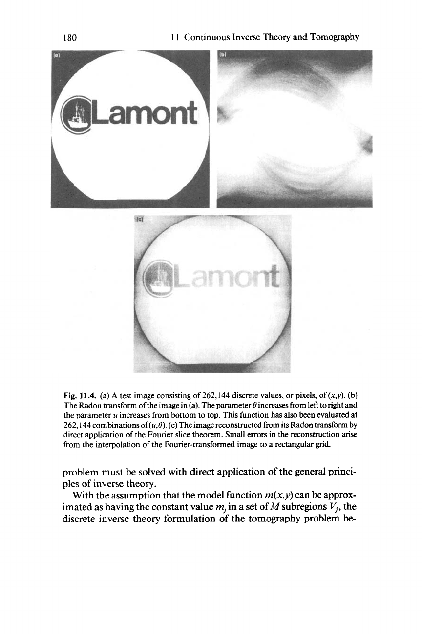
Fig.

11.4. (a)

test image consisting of

262,144

discrete values,

pixels, of

(x,y).

(b)

The Radon transform ofthe image

(a). The parameter

increases from left to right and

the parameter

increases from bottom to top. This function has also

been

evaluated

262,144

combinations of(u,0). (c) The image reconstructed from

its

Radon transform by

direct application of the Fourier slice theorem. Small errors

the reconstruction

arise

from the interpolation of the Fourier-transformed image to a rectangular grid.

problem must be solved with direct application of the general princi-

ples

inverse theory.

With the assumption that the model function

m(x,y)

can

approx-

imated as having the constant value

in a set

subregions

V,,

the

discrete inverse theory formulation of the tomography problem

be-

11.7

Backprojection

181

comes

XjG,mj,

where the data kernel

gives the arc length of

the ith ray in the jth subregion. In a typical tomography problem, there

may be tens of thousands of subregions

lo4) and millions of rays

lo6),

the data kernel is a very large matrix. (The data kernel is,

however, sparse, since a given ray will not traverse very many of the

subregions.) The solution of the problem directly by, say, the least

squares formula

[GTG]-lGTd may

impractical, owing to the

difficulty of directly inverting the large

matrix [GTG]. One

alternative to direct inversion is “backprojection,” an iterative method

for solving a system

linear equations that is similar to the well-

known Gauss- Seidel and Jacobi methods of linear algebra.

We begin by writing the data kernel as

hiF,,

where

is the

length of the ith ray and

is the fractional length of the ith ray in the

jth subregion. The basic equation of the tomography problem is then

X,F,mj

di, where

di/hi.

The least squares solution is

[FTF]m

FTd’

FTF]m

FTd’

1.23)

rn&

FTd’

FTF]m&

Note that we have both added and subtracted the identity matrix in the

second step. The trick is now to use this formula iteratively, with the

previous estimate ofthe model parameters on the right-hand side ofthe

equation:

m=t(i)

FTd’

FTF]m&(i-l) (1 1.24)

Here mcllt(i)is the

rn&

after the ith iteration. When the iteration is started

with

m&(O)

then

(11.25)

This formula has a simple interpretation which earns it the name

backprojection. In order to bring out this interpretation, we will sup

pose that this is an acoustic tomography problem,

that the model

parameters correspond to acoustic slowness (reciprocal velocity) and

the

data

to acoustic travel time. Suppose that there are only one ray

and one subregion

1).

Then the slowness

this subre-

gion would

estimated

d, /h

that is,

travel time divided

by ray length. If there are several subregions, then the travel time is

distributed equally (“backprojected”) among them,

that those with

182

Continuous

Inverse

Theory

and

Tomography

the shortest ray lengths

are assigned the largest slowness. Finally, if

there are several rays, a given model parameter’s total slowness is just

the sum of the estimates for the individual rays. This last step is quite

unphysical and causes the estimates of the model parameters to grow

with the number of rays. Remarkably, this problem introduces only

long-wavelength errors into the image,

that a high-pass-filtered ver-

sion of the image can often

quite useful. In many instances the first

approximation in Eq.

(

1.24)

is satisfactory, and further iterations

need not

performed. In other instances, iterations are necessary.

further complication arises in practical tomography problems

when the ray path is itself a function of the model parameters (such as

in acoustic tomography, where the acoustic velocity structure deter-

mines the ray paths). The procedure here

to write the model as a

small perturbation

drn(x,y)

about a trial or “background”

rn(x,y)

rno(x,y)

drn(x,y).

The tomoraphy problem for drn and rays based on

rn,

is solved using standard methods, new rays are determined for the

new structure, and the whole process it iterated. Little is known about

the convergence properties of such an iteration, except perhaps when

there is an underlying reason to believe that the data are relatively

insensitive to small errors in the model (such

is given by Fermat’s

principle in acoustics).

SAMPLE INVERSE

PROBLEMS

12.1

Image Enhancement Problem

Suppose that a camera moves slightly during the exposure

photograph

(so

that the picture is blurred) and that the amount and

direction

motion are known. Can the photograph

“unblurred”?

For simplicity we shall consider a one-dimensional camera (that is,

one that records brightness along a line) and assume that the camera

moves parallel to the line. The camera is supposed to be

the digital

type; it consists

a row

light-sensitive elements that measure the

total amount

light received during the exposure. The data

are a set

numbers that represent the amount

light recorded at each

camera “pixels.” Because the scene’s brightness varies continuously

along the line

the camera, this is properly a problem in continuous

inverse theory. We shall discretize it, however, by assuming that the

scene can be adequately approximated

a row

small square

elements, each with a constant brightness. These elements

form

model parameters

mi.

Since the camera’s motion is known, it is

183

184

Sample Inverse Problems

...

111

possible to calculate each scene element’s relative contribution to the

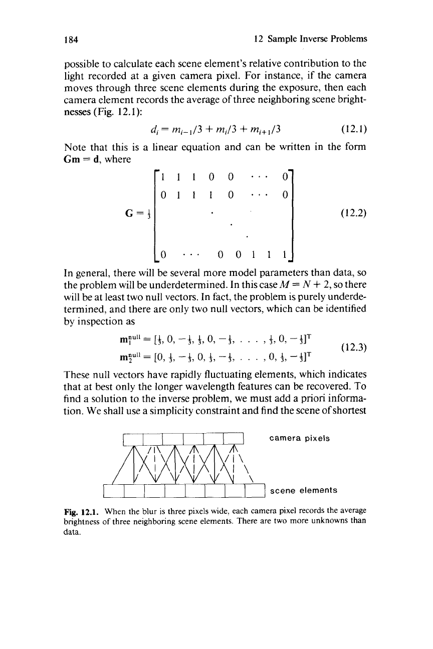
light recorded at a given camera pixel. For instance, if the camera

moves through three scene elements during the exposure, then each

camera element records the average of three neighboring scene bright-

nesses

(Fig.

12.1):

mi-,/3

mi/3

m,+,/3

(12.1)

Note that this

a linear equation and can be written in the form

where

100

110

(12.2)

In general, there will be several more model parameters than data,

the problem will be underdetermined. In this case

there

will be at least two null vectors. In fact, the problem

purely underde-

termined, and there are only two null vectors, which can be identified

by inspection as

These null vectors have rapidly fluctuating elements, which indicates

that at best only the longer wavelength features can be recovered. To

find a solution to the inverse problem, we must add a priori informa-

tion. We shall use a simplicity constraint and find the scene of shortest

camera pixels

scene elements

Fig.

12.1.

When the blur

three pixels wide, each camera pixel records the average

brightness

three neighboring scene elements. There are two

unknowns than

data.

12.1

Image Enhancement

Problem

185

scene element

camera pixel

(C)

scene element

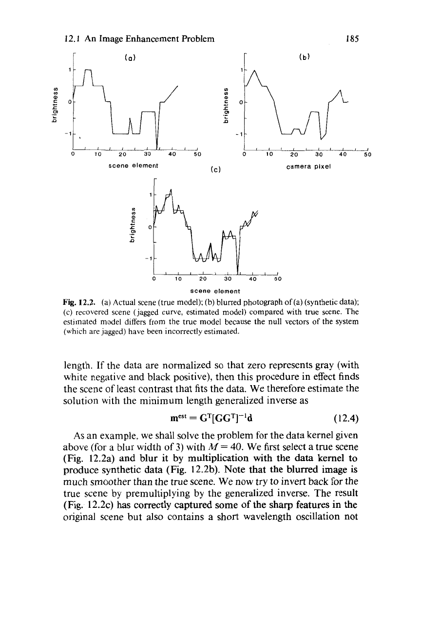
Fig.

12.2.

(a) Actual scene (true model);

(b)

blurred photograph of(a) (synthetic data);

estimated model differs from the true model because the

null

vectors

the system

(which are jagged) have been incorrectly estimated.

length.

the data are normalized

that zero represents gray (with

white negative and black positive), then this procedure in effect finds

the scene of least contrast that fits the data. We therefore estimate the

solution with the minimum length generalized inverse as

GT[

GGT]-'d

(12.4)

an example, we shall solve the problem for the data kernel given

above (for a blur width of

with

40.

We first select a true scene

(Fig. 12.2a) and blur it

multiplication with the data kernel to

produce synthetic data (Fig. 12.2b). Note that the blurred image

much smoother than the true scene. We now

try

invert back for the

true scene by premultiplying by the generalized inverse. The result

(Fig. 12.2~) has correctly captured some of the sharp features in the

original scene but also contains a short wavelength oscillation not

mest

186

Sample Inverse Problems

present in the true scene. This error results from creating a recon-

structed scene containing an incorrect combination of null vectors.

In this example, the generalized inverse is computed by simply

performing the given matrix multiplications on a computer and then

inverting

[GGT]

Gauss-

Jordan reduction with partial pivoting (see

Section

13.2).

It is possible, however, to deduce the

form

[GGT]

analytically since

has a simple structure.

typical row contains the

sequence

In this problem, which deals

with small

(40

42)

matrices, the effort saved is negligible. In more

complicated inverse problems, however, considerable savings can

result from a careful analytical treatment of the structures of the

various matrices.

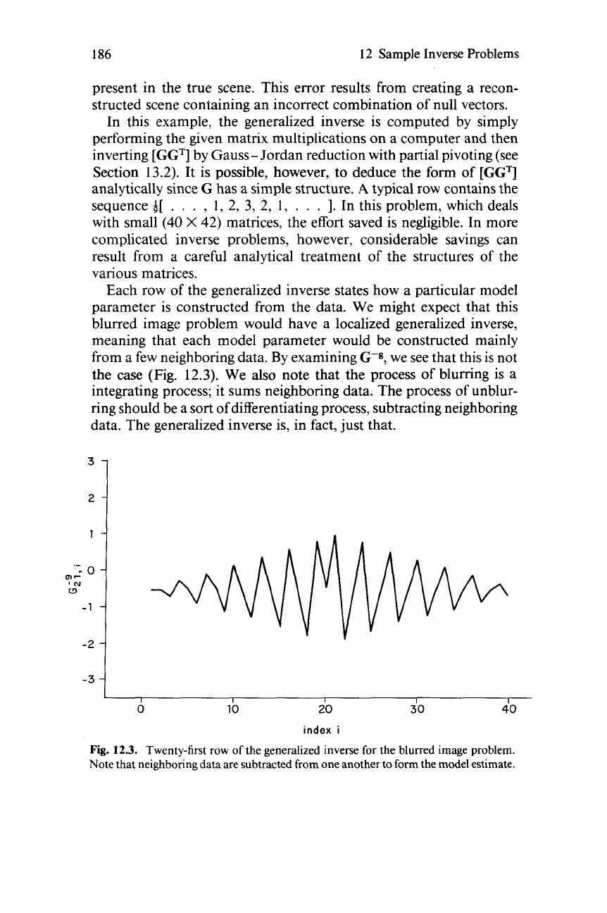
Each row

the generalized inverse states how a particular model

parameter is constructed from the data. We might expect that this

blurred image problem would have a localized generalized inverse,

meaning that each model parameter would be constructed mainly

from a few neighboring data.

examining

G-g,

we see that this is not

the case (Fig.

12.3).

also

note that the process of blumng is a

integrating process; it sums neighboring data. The process of unblur-

ring should be a

sort

differentiating process, subtracting neighboring

data. The generalized inverse is, in fact, just that.

-3

-1

index

Fig.

12.3.

Twenty-first row

the generalized inverse

for

the blurred image problem.

Note that neighboring data are subtracted

from

one another to

form

the model estimate.

12.2

Digital

Filter

Design

187

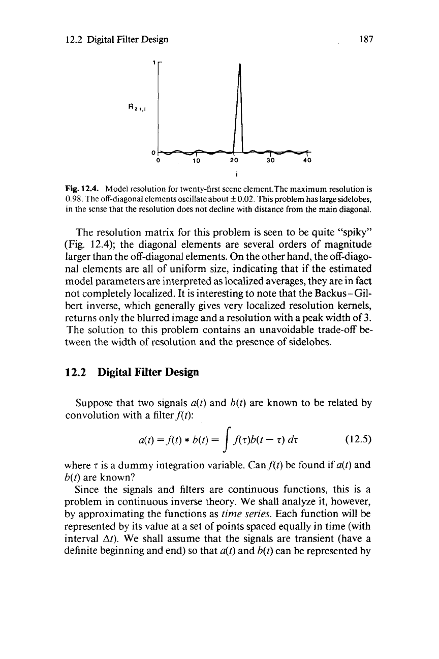
Fig.

12.4.

Model resolution

for

twenty-first scene element.The maximum resolution is

0.98.

The off-diagonal elements oscillate about

0.02.

This problem has large sidelobes,

in the sense that the resolution does not decline with distance from the main diagonal.

The resolution matrix for this problem is seen to be quite “spiky”

(Fig.

12.4);

the diagonal elements are several orders of magnitude

larger than the off-diagonal elements. On the other hand, the off-diago-

nal elements are all of uniform size, indicating that if the estimated

model parameters are interpreted as localized averages, they are in fact

not completely localized. It is interesting to note that the Backus-Gil-

bert inverse, which generally gives very localized resolution kernels,

returns only the blurred image and a resolution with a peak width of

The solution to this problem contains an unavoidable trade-off be-

tween the width of resolution and the presence of sidelobes.

12.2

Digital Filter Design

Suppose that two signals

a(t)

and

b(t)

are known to be related by

convolution with a filterf(t):

a(t)

=f(t)

b(t)

f(t)b(t

2.5)

where

is a dummy integration variable. Canf(t) be found

a(t)

and

b(t)

are known?

Since the signals and filters are continuous functions, this is a

problem in continuous inverse theory. We shall analyze it, however,

by approximating the functions as

time

series.

Each function will be

represented by its value at a set of points spaced equally in time (with

interval

At).

We shall assume that the signals are transient (have a

definite begnning and end)

that

a(t)

and

b(t)

can be represented by