Menke W. Geophysical Data Analysis: Discrete Inverse Theory
Подождите немного. Документ загружается.

138
8
Non -Gaussian Distributions
8.4
Solving
L,
Norm
Problems
We shall show that this problem can be transformed into a “linear
programming” problem, a type that has been studied intensively and
for which means of solution are known (e.g., the so-called Simplex
algorithm; see Section
12.7).
The linear programming problem can be
stated as follows:
Find the
x
that maximizes
z
=
cTx
subject to the constraints
This problem was first studied by economists and business operations
analysts. For example,
z
might represent the profit realized
by
a factory
producing a product line, where the number
of
each product is given
by
x
and the profit on each item given by
c.
The problem is to
maximize the total profit
z
=
cTx
without violating the constraint that
one can produce only a positive amount of each product, or any other
linear inequality constraints that might represent labor laws, union
regulations, physical limitation of machines, etc. Computer programs
that can solve the linear programming problem are readily available.
First, we shall consider the completely underdetermined linear
problem with a priori model parameters, mean
(m),
and variance
a;.
The problem is to minimize the weighted length
L
=
c
[mi
-
(m,)la,f
subject to the constraint
Gm
=
d.
We first introduce 5Mnew variables
m:,
m”,,
a,,
x,,
and
x:,
where
i
=
1,
. . .
,
M.
The linear program-
ming problem may be stated as follows [Ref.
61:
Minimize
C
a,a;f
subject to the constraints
G[m’
-
m”]
=
d
[mi
-
my]
+
xi
-
ai
=
(mi)
[mi
-
my]
-
x;
+
ai
=
(mi)
mi20
my20
ai
2
0
XI
2
0
xi20
(8.10)
This linear programming problem has
5M
unknowns and
8.4
Solving
L,
Norm
Problems
139
N
+
2M constraints.
If
one makes the identification
m
=
m'
-
m",
signs of the elements of
m
are not constrained even though those of
m'
and
m"
are. Note that the remaining constraints can be rewritten as
a;
-
x;
=
[m;
-
(mi)]
a.
I1
-
x!
=
-
[m;
-
(mi)]
(8.11)
where the
a,,
x,,
and
xi
are nonnegative. Now
if
[m,
-
(m,)]
is posi-
tive, the first equation requires
a,
2
[m,
-
(m,)]
since
x,
cannot be
negative. The second constraint can always be satisfied by choosing
some appropriate
xi.
On the other hand, if
[m,
-
(m,)]
is negative,
then the first constraint can always be satisfied by choosing some
appropriate
x,
but the second constraint requires that
a,
2
-
[m,
-
(m,)].
Taken together, these two constraints imply that
a,
2
[[m,
-
(m,)]l.
Minimizing
X
a,a;f
is therefore equivalent to minimiz-
ing the weighted solution length
L.
The
L,
minimization problem has
been converted to a linear programming problem.
The completely overdetermined problem can be converted into a
linear programming problem in a similar manner. We introduce
2M+ 3Nnew variables, mi, mi',
i
=
1,
Mand
a,,
x,,
xi,
i
=
1,
Nand
2N constraints. The equivalent linear programming problem
is
[Ref.
61:
Minimize
z
aia;,'
subject to the constraints
z
Gij[m(
-
my]
+
xi
-
=
d,
(8.12)
The mixed-determined problem can be solved by any of several
methods. By analogy to the
L,
methods described in Chapters 3 and
7,
we could either pick some a priori model parameters and minimize
E
+
L,
or try to separate the overdetermined model parameters from
the underdetermined ones and apply a priori information to the
underdetermined ones only. The first method leads to a linear pro-
gramming problem similar to the two cases stated above but with even
140
8
Non -Gaussian Distributions
more variables
(5M
+
3N)
and constraints
(2M
+
2N):
Minimize
C
a,a&f
+
C
a:ozl
subject to the constraints
(8.13)
The second method is more interesting. We can use the singular-
value decomposition to identify the null space of
G.
The solution then
has the form
P
M
1-
I
I-pi
1
mest
=
c.
u,vp,
+
C
b,v,,
=
Vpa
+
Vob
(8.14)
where the
v’s
are the model eigenvectors from the singular-value
decomposition and
a
and
b
are vectors with unknown coefficients.
Only the vector
a
can affect the prediction error,
so
one uses the
overdetermined algorithm to determine it:
find
aest
that minimizes
E
=
Ild
-
Gmll,
=
Id,
-
[UpApal,la;,l
1
(8.15)
Next, one uses the underdetermined algorithm to determine
b:
find
best
that minimizes
M
L
=
Ilm
-
(m)II
=
a;tI[V,b],
-
(mi
-
[Vpaest],)l
(8.16)
I==
1
It is possible to implement the basic underdetermined and overdeter-
mined
L,
algorithms in such a manner that the many extra variables
are never explicitly calculated [Ref.
61.
This procedure vastly decreases
the storage and computation time required, making these algorithms
practical for solving moderately large
(M
=
100)
inverse problems.
8.5
TheL,Norm
141
8.5
The
L,
Norm
While the
L,
norm weights “bad” data less than the
L2
norm, the
L,
norm weights it more:
The prediction error and solution length are weighted by the reciprocal
of their a priori standard deviations. Normally one does not want to
emphasize outliers,
so
the
L,
form is useful mainly in that it can
provide a “worst-case” estimate of the model parameters for compari-
son with estimates derived on the basis of other norms. If the estimates
are in fact close to one another, one can be confident that the data are
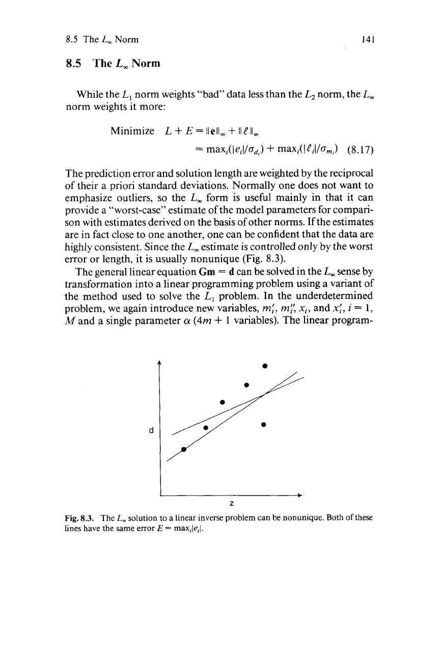
highly consistent. Since the
L,
estimate is controlled only by the worst
error or length, it is usually nonunique (Fig.
8.3).
The general linear equation
Gm
=
d
can be solved in the
L,
sense by
transformation into a linear programming problem using a variant of
the method used to solve the
L,
problem. In the underdetermined
problem, we again introduce new variables,
rn:,
rnl:
xi,
and
x:,
i
=
1,
M
and a single parameter
a
(4m
+
1
variables). The linear program-
Z
Fig.
8.3.
The
L,
solution to a linear inverse problem can be nonunique. Both
of
these
lines have the same error
E
=
max,le,l.

142
8
Non -Gaussian Distributions
ming problem is
Minimize
a
subject to the constraints
G[m’
-
m”]
=
d
[mi
-
m:’]
+
x,
-
aam,
=
(m,)
(8.18)
[mi
-
my3
-
x:
+
aam,
=
(m,)
m:ro
m:’20
a20
x,rO
xi20
where m
=
m’
-
m”.
We note that the new constraints can be written
as
(8.19)
where
a,
x,
,
and
xi
are nonnegative. Using the same argument as was
applied in the
L,
case, we conclude that these constraints require that
a
2
[[m,
-
(m,)]/o,,l
for all
i.
Since this problem has but a single
parameter
a,
it must therefore satisfy
a
2
max,(l[m,
-
(mi>l/am,l>
(8.20)
Minimizing
CII
yields the
L,
solution. The linear programming prob-
lem for the overdetermined case
is
Minimize
a
subject to the constraints
(8.21)
mi”
0
my20
a20
xi20
x;ro
The mixed-determined problem can be solved by applying these
algorithms and either of the two methods described for the
L,
problem.
NONLINEAR INVERSE
PROBLEMS
9.1
Parameterizations
In setting up any inverse problem, it is necessary to choose variables
to represent data and model parameters (to select a parameterization).
In many instances this selection is rather ad hoc; there might be no
strong reasons for selecting one parameterization over another. This
can become a substantial problem, however, since the answer obtained
by solving an inverse problem is dependent on the parameterization.
In other words, the solution is not invariant under transformations of
the variables. The exception is the linear inverse problem with Gaus-
sian statistics, in which solutions are invariant for any linear repa-
rameterization of the data and model parameters.
As
an illustration of this difficulty, consider the problem of fitting a
straight line to the data pairs
(1,
I),
(2,2),
(3,3),
(4,5).
Suppose that we
regard these data as
(z,
d)
pairs where
z
is an auxiliary variable. The
least squares
fit
is
d
=
-0.500
+
1.3002.
On
the other hand, we might
regard them as
(d’,
z’)
pairs where
z’
is the auxiliary variable. Least
143
144
9
Nonlinear Inverse
Problems
squares then gives
d’
=
0.309
+
0.743z’, which can be rearranged as
z’
=
-0.416
+
1.345d’. These two straight lines have slopes and
intercepts that differ by about
20%.
This discrepancy arises from two sources. The first is an inconsistent
application of probability theory. In the example above we alternately
assumed that
z
was exactly known and
d
followed Gaussian statistics
and that
z
=
d’
followed Gaussian statistics and
d
=
z’
was exactly
known. These are two radically different assumptions about the distri-
bution of errors,
so
it
is
no wonder that the solutions are different.
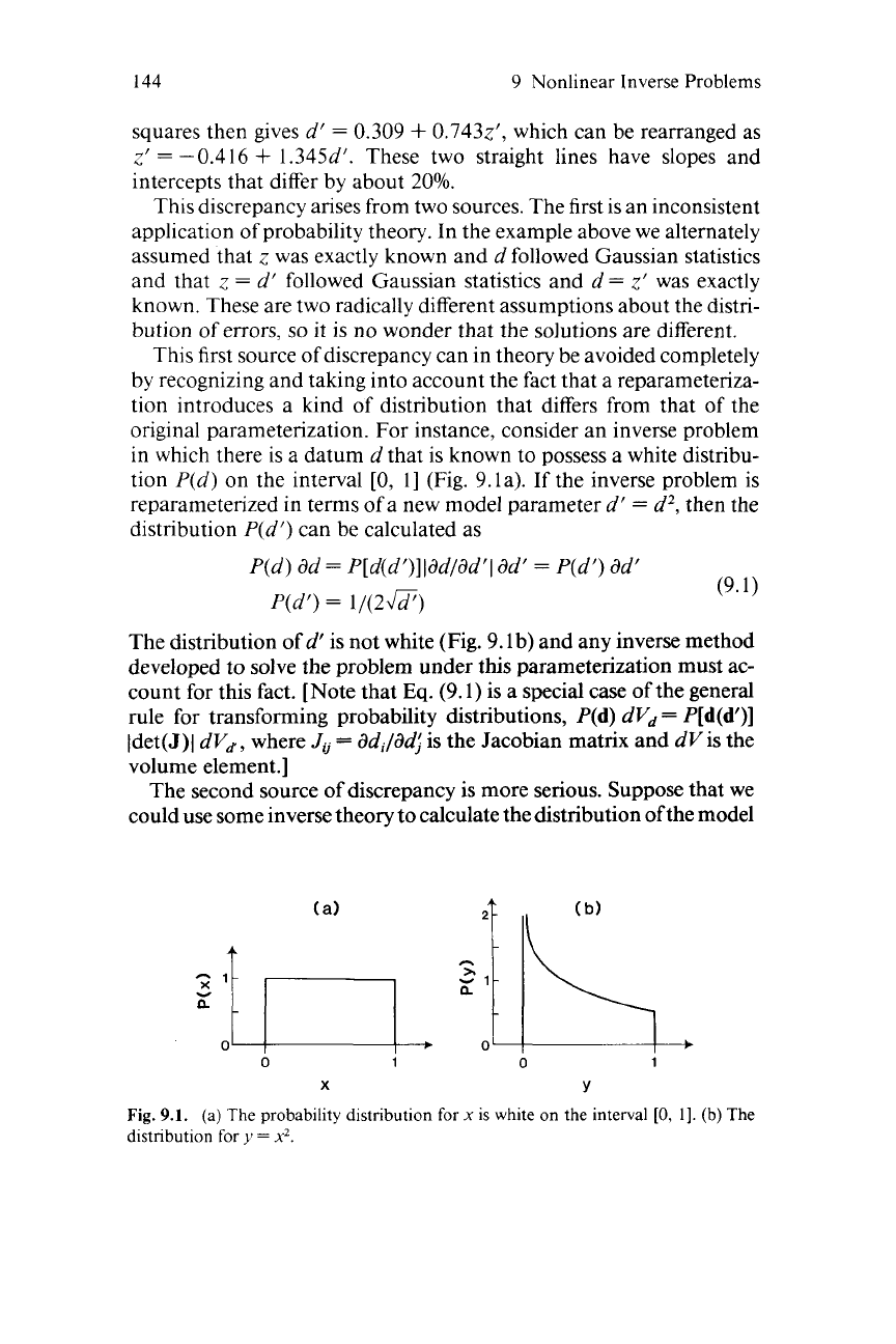
This first source of discrepancy can in theory be avoided completely
by recognizing and taking into account the fact that a reparameteriza-
tion introduces a kind of distribution that differs from that of the
original parameterization. For instance, consider an inverse problem
in which there is a datum
d
that is known to possess a white distribu-
tion
P(d)
on the interval
[0,
I] (Fig. 9.1a).
If
the inverse problem is
reparameterized in terms
of
a new model parameter
d’
=
d2,
then the
distribution
P(d’)
can be calculated as
P(d)
dd
=
P[d(d’)]ldd/dd’I
ad‘
=
P(d’)
dd‘
(9.1)
P(d’)
=
1/(2G)
The distribution of
d’
is not white (Fig. 9. lb) and any inverse method
developed to solve the problem under this parameterization must ac-
count for this fact. [Note that
Eq.
(9.1) is a special case of the general
rule for transforming probability distributions, P(d)
dVd
=
P[d(d’)]
Idet(J)I
dVd,
where
JU
=
dd,/dd,l
is the Jacobian matrix and
dVis
the
volume element.]
The second source of discrepancy is more serious. Suppose that we
could use some inverse theory to calculate the distribution ofthe model
21
1
I
(a)
I
,
?)
i\
).
Y
n
0
0
1
0
1
X
Y
Fig.
9.1.
(a)
The
probability distribution
for
x
is white
on
the interval
[0,
11.
(b) The
distribution
for
y
=
x2.
9.1
Parameterizations
145
parameters under a particular parameterization. We could then use
Eq.
(9.1)
to find
theirdistributionunderanyarbitraryparameterization.
Insofar as the distribution of the model parameters
is
the answer to the
inverse problem, we would have the correct answer in the new parame-
terization. Probability distributions are invariant under changes of
parameterization. However, a distribution is not always the answer for
which we are looking. More typically, we need an estimate (a single
number) based on a probability distribution (for instance, its maxi-
mum likelihood point or mean value).
Estimates are not invariant under changes in the parameterization.
For example, suppose
P(m)
has a white distribution as above. Then
if
m’
=
m2,
P(m’)
=
1/(2&2).
The distribution in
m
has no maximum
likelihood point, whereas the distribution in
m’
has one at
m’
=
m
=
0.
The distributions also have different means (expectations)
E:
E[~I
=
m~(m)
am
=
m
am
=
4
E[m‘]
=
m’P(m’)
am’
=
I
+&2
amf
=
4
Even though
m’
equals the square of the model parameter
m,
the
expectation of
m’
is not equal to the square of the expectation of
m:
There is some advantage, therefore, in working explicitly with
probability distributions as long as possible, forming estimates only at
the last step.
If
m
and
m’
are two different parameterizations of model
parameters, we want to avoid as much as possible sequences like
distribution for
m
-
estimate of
m
-
estimate of
m’
I
(9.2)
I’ I’
I
4
+
(:I2.
in favor of sequences like
distribution for
m
-
distribution for
m’
__*
estimate of
rn’
Note, however, that the mathematics for this second sequence
is
typically much more difficult than that for the first.
There are objective criteria for the “goodness” of a particular esti-
mate of a model parameter. Suppose that we are interested in the value
of a model parameter
m.
Suppose further that this parameter either
is
deterministic with a true value or (if it is a random variable) has a
well-defined distribution from which the true expectation could be
calculated if the distribution were known. Of course, we cannot know
the true value; we can only perform experiments and then apply
146
9
Nonlinear Inverse Problems
inverse theory to derive an estimate of the model parameter. Since any
one experiment contains noise, the estimate we derive will not coin-
cide with the true value
of
the model parameter. But we can at least
expect that if we perform the experiment enough times, the estimated
values will scatter about the true value. If they do, then the method of
estimating is said to be
unbiased.
Estimating model parameters by
taking nonlinear combinations of estimates of other model parameters
almost always leads to bias.
d
0.001
I
I I
0
5
10
15 20
L
log
d
-
L
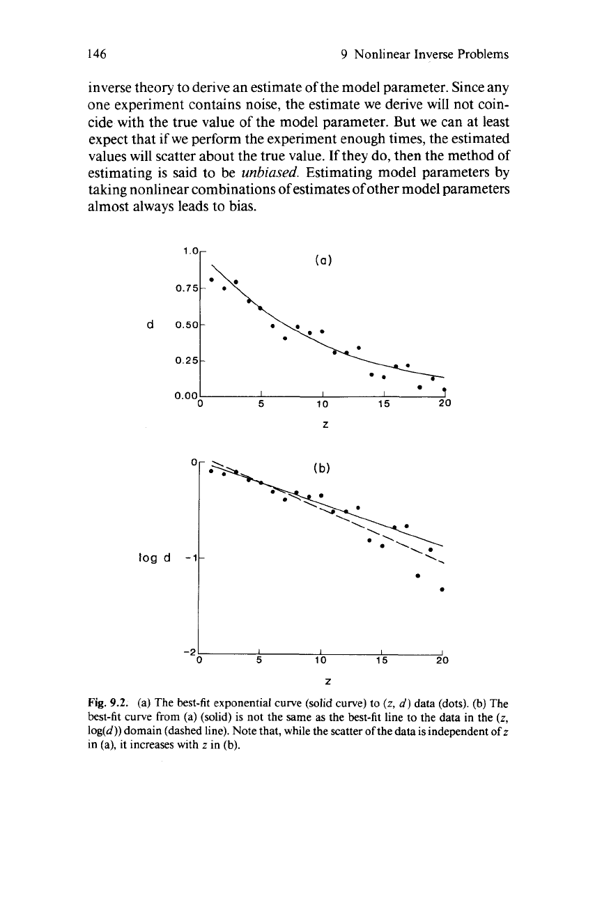
Fig.
9.2.
(a) The best-fit exponential curve (solid curve) to
(z,
d)
data (dots).
(b)
The
best-fit curve from (a) (solid) is not the same as the best-fit line to the data in the
(z,
log(d)) domain (dashed line). Note that, while the scatter of the data is independent of z
in (a), it increases with
z
in
(b).
9.3
The Nonlinear Inverse Problem with Gaussian Data
147
9.2
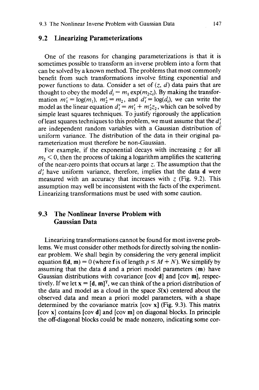
Linearizing Parameterizations
One of the reasons for changing parameterizations is that it is
sometimes possible to transform an inverse problem into a form that
can be solved by a known method. The problems that most commonly
benefit from such transformations involve fitting exponential and
power functions to data. Consider a set of
(z,
d)
data pairs that are
thought to obey the model
di
=
m,
exp(m2zi). By making the transfor-
mation
m;
=
log(m,),
m;
=
m2,
and
dj=
log(di), we can write the
model as the linear equation
di
=
m{
+
m;z2,
which can be solved by
simple least squares techniques. To justify rigorously the application
of least squares techniques to this problem, we must assume that the
dj
are independent random variables with a Gaussian distribution of
uniform variance. The distribution of the data in their original pa-
rameterization must therefore be non-Gaussian.
For example,
if
the exponential decays with increasing
z
for all
m2
<
0,
then the process of taking a logarithm amplifies the scattering
of the near-zero points that occurs at large
z.
The assumption that the
dj
have uniform variance, therefore, implies that the data
d
were
measured with an accuracy that increases with
z
(Fig.
9.2).
This
assumption may well be inconsistent with the facts of the experiment.
Linearizing transformations must be used with some caution.
9.3
The Nonlinear Inverse Problem with
Gaussian Data
Linearizing transformations cannot be found for most inverse prob-
lems. We must consider other methods for directly solving the nonlin-
ear problem. We shall begin by considering the very general implicit
equation
f(d, m)
=
0
(where
f
is of length
p
5
M
+
N).
We simplify by
assuming that the data
d
and a priori model parameters
(m)
have
Gaussian distributions with covariance [cov
d]
and [cov
m],
respec-
tively. If we let
x
=
[d, mIT,
we can think of the a priori distribution of
the data and model as a cloud in the space
S(x)
centered about the
observed data and mean a priori model parameters, with a shape
determined by the covariance matrix [cov
x]
(Fig.
9.3).
This matrix
[cov
x]
contains [cov
d]
and [cov
m]
on diagonal blocks. In principle
the off-diagonal blocks could be made nonzero, indicating some cor-