Menke W. Geophysical Data Analysis: Discrete Inverse Theory
Подождите немного. Документ загружается.

This page intentionally left blank
7
APPLICATIONS
OF
VECTOR SPACES
7.1
Model and Data Spaces
We have used vector notation for the data
d
and model parameters
m
mainly because it facilitates the algebra. The concept of vectors can
also be used to gain insight into the properties of inverse problems. We
therefore introduce the idea of vector spaces containing
d
and
m,
which we shall denote
S(d)
and
S(m).
Any particular choice of
m
and
d
is then represented as a vector in these spaces (Fig.
7.1).
The linear equation
Gm
=
d
can be interpreted as a mapping of
vectors from
S(m)
to
S(d)
and its solution
mest
=
G-pd
as a mapping of
vectors from
S(d)
to
S(m).
One important property of a vector space is that its coordinate axes
are arbitrary. Thus far we have been using axes parallel to the individ-
ual model parameters, but we recognize that we are by no means
required to do
so.
Any set of vectors that spans the space will serve as
coordinate axes. The Mth dimensional space
S(m)
is spanned by any
A4 vectors, say,
m,
,
as long as these vectors are linearly independent.
109
110
7
Applications
of
Vector Spaces
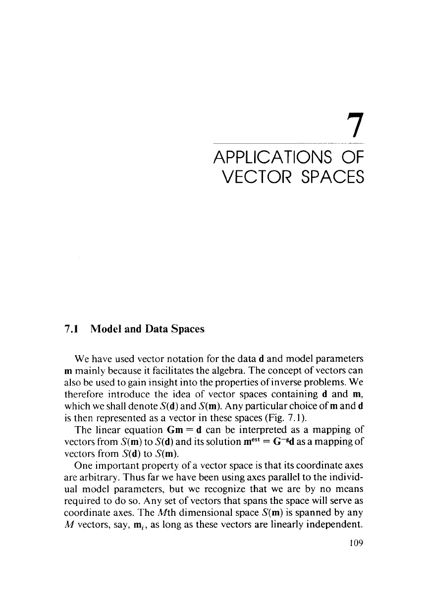
Fig.
7.1.
(a) The model parameters represented as a vector
m
in the M-dimensional
space
S(m)
of
all possible model parameters.
(b)
The data represented as a vector
d
in the
N-dimensional space
S(d)
of
all possible data.
An arbitrary vector lying in
S(m),
say
m*,
can be expressed as a sum of
these
A4
basis vectors, written as
M
m*
=
aimi
i=
1
(7.1)
where the
a’s
are the components of the vector
m*
in the new
coordinate system.
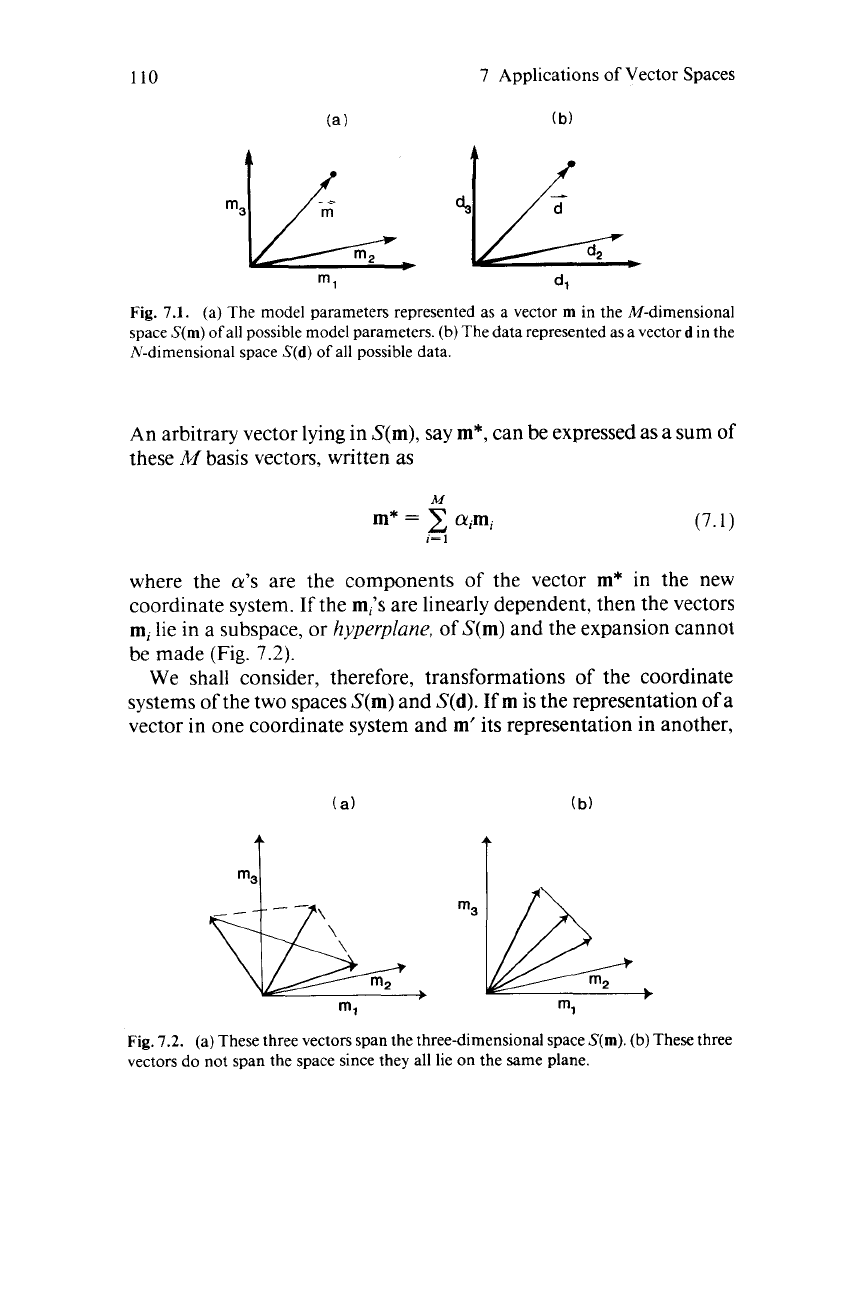
If
the
m,’s
are linearly dependent, then the vectors
m,
lie in a subspace, or
hyperplane,
of
S(m)
and the expansion cannot
be made (Fig.
7.2).
We shall consider, therefore, transformations of the coordinate
systems of the two spaces
S(m)
and
S(d).
If
m
is the representation
of
a
vector in one coordinate system and
m’
its representation in another,
t
t
Fig.
7.2.
(a) These three vectors span the three-dimensional space
S(m).
(b)
These three
vectors do not span the space since they all lie
on
the same plane.
7.2
Householder
Transformations
111
we can write the transformation as
m’=Tm
and
m=T-’m’
(7.2)
where
T
is the transformation matrix.
If
the new basis vectors are still
unit vectors, then
T
represents simple rotations or reflections of the
coordinate axes.
As
we shall show below, however, it is sometimes
convenient‘to choose a new set of basis vectors that are not unit
vectors.
7.2
Householder Transformations
In this section we shall show that the minimum length, least squares,
and constrained least squares solutions can be found through simple
transformations of the equation
Gm
=
d.
While the results are identi-
cal to the formulas derived in Chapter
3,
the approach and emphasis
are quite different and will enable us to visualize these solutions in a
new way. We shall begin by considering a purely underdetermined
linear problem
Gm
=
d
with
M>
N.
Suppose we want to find the
minimum length solution (the one that minimizes
L
=
mTm).
We
shall show that it is easy to find this solution by transforming the model
parameters into a new coordinate system
m’
=
Tm.
The inverse prob-
lem becomes
d
=
Gm
=
GIm
=
GT-ITm
=
{GT-’}(Tm}
=
G’m’
(7.3)
where
G’
=
GT’
is the data kernel in the new coordinate system. The
solution length becomes
L
=
mTm
=
(T--lm’)T(T-Im’)
=
m’T(T-lTT-’)m’
(7.4)
Suppose that we could choose
T
so
that
(T-ITT-’)
=
I.
The solution
length would then have the same form in both coordinate systems,
namely, the sum of squares of the vector elements. Minimizing
mlTrn’
would be equivalent to minimizing
mTm.
Transformations of this type
that do not change the length of the vector components are called
unitary transformations.
They may be interpreted as rotations and
reflections of the coordinate axes. We can see from Eq. (7.4) that
unitary transformations satisfy
TT
=
T-I.
Now suppose that we could also choose the transformation
so
that
112
7
Applications
of
Vector Spaces
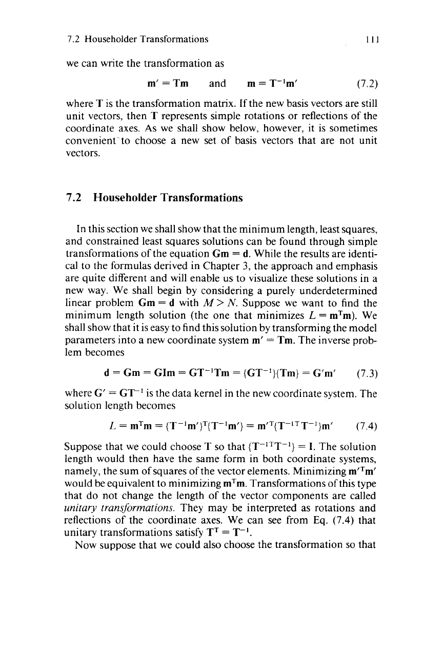
G'
is the lower triangular matrix
......
G;,
0
0 0
...
0
0
G;,
Gi2
0
0
...
0
0
G;,
Ci2
G;,
0
...
0
0
......
......
..
Gh,
Gh2
Gh,
Gh4
...
GLN
0
...
0
(7.5)
Notice that no matter what values we pick for
(m:est,
i
=
N
+
1,
M),
we'cannot change the value of
G'm'
since the last
M
-
N
columns of
G'
are all zero. On the other hand, we can solve for the first Nelements
of
mlest
uniquely as
This process is known as
back-solving.
Since the first
N
elements of
dest
are thereby determined,
m"m'
can
be
minimized by setting the
remaining
m:est
equal to zero. The solution in the original coordinate
system is then
mest
=
T-'mtest.
Since this solution satisfies the data
exactly and minimizes the solution length, it is equal to the minimum-
length solution (Section 3.7).
One such transformation that can triangularize a matrix is called a
Householder transformation.
We shall discuss in Section 7.3 how such
transformations can be found. We employ a transformation process
that separates the determined and undetermined linear combinations
of model parameters into two distinct groups
so
that we can deal with
them separately. It is interesting to note that we can now easily
determine the null vectors for the inverse problem. In the transformed
coordinates they are the set of vectors whose first
N
elements are zero
and whose last
M
-
N
elements are zero except for one element. There
are clearly
M
-
N such vectors,
so
we have established that there are
never more than Mnull vectors in a purely underdetermined problem.
7.2
Householder Transformations
113
The null vectors can easily be transformed back into the original
coordinate system by premultiplication by
T-I.
Since all but one
element of the transformed null vectors are zero, this operation
just
selects a column of
T-’,
(or, equivalently, a row of
T).
As
we shall see below, Householder transformations have applica-
tion to a wide variety of methods that employ the
L,
norm
as
a
measure of size. These transformations provide an alternative method
of solving such problems and additional insight into their structure.
They also have computational advantages that we shall discuss in
Section
12.3.
The overdetermined linear inverse problem
Gm
=
d
with
N
>
M
can also be solved through the use of Householder transformations. In
this case we seek a solution that minimizes the prediction error
E
=
e’e.
We seek a transformation with two properties: it must oper-
ate on the prediction error
e (e’
=
Te)
in such
a
way that minimizing
elTe’
is the same as minimizing
eTe,
and it must transform the data
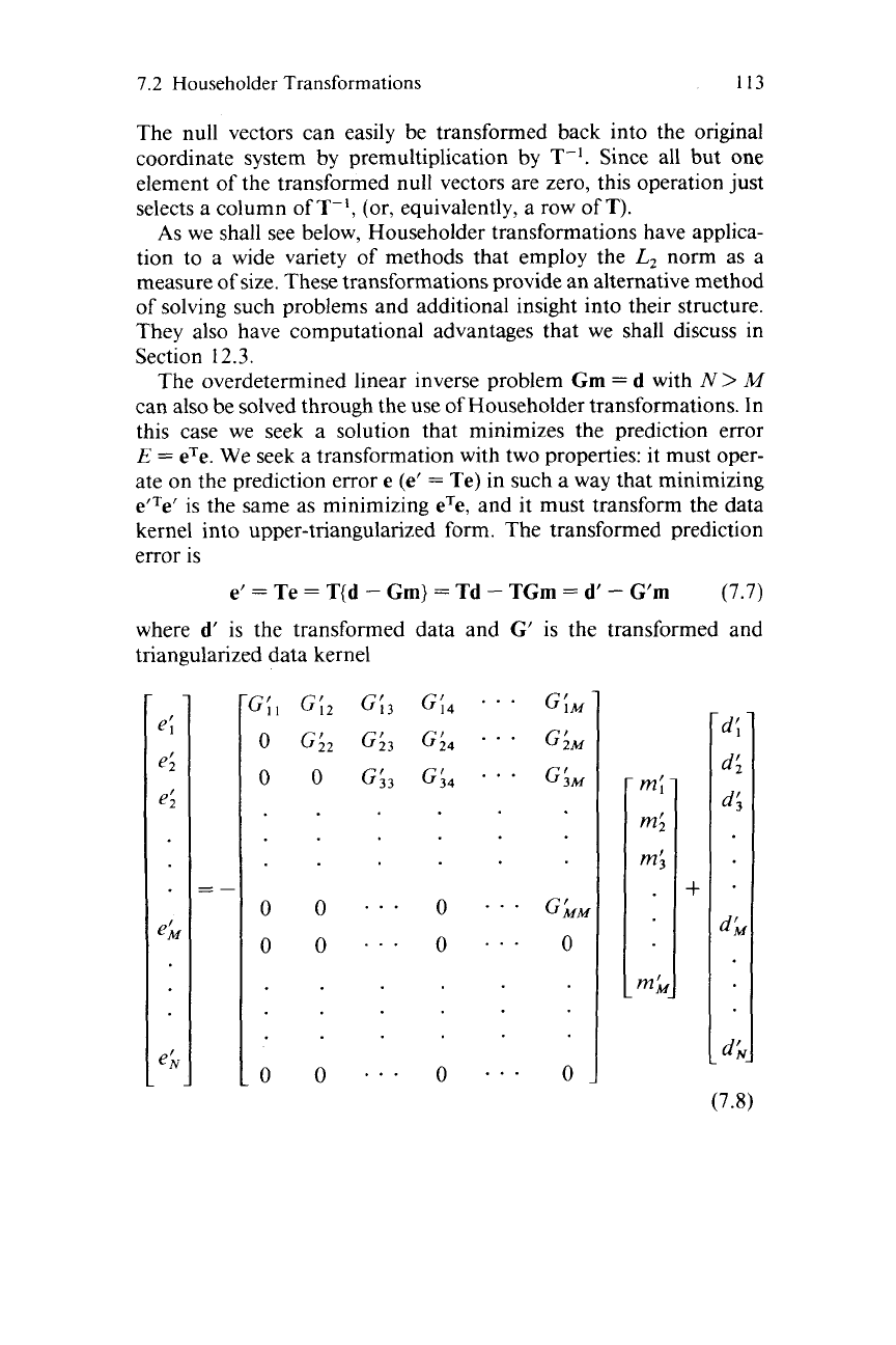
kernel into upper-triangularized form. The transformed prediction
error is
e’
=
Te
=
T(d
-
Gm)
=
Td
-
TGm
=
d’
-
G’m
(7.7)
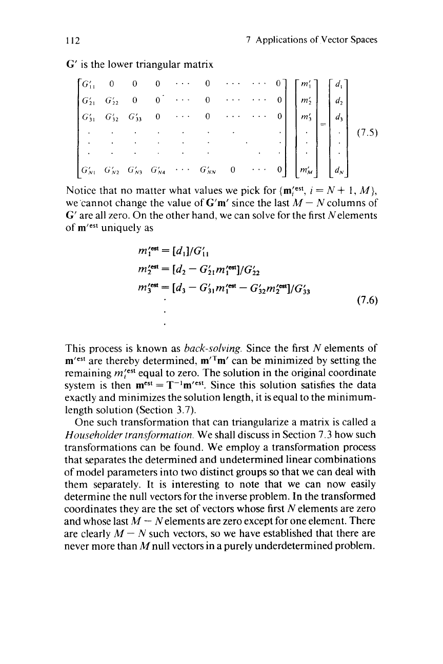
where
d‘
is the transformed data and
G’
is the transformed and
triangularized data kernel
GL3
0
0
0
...
0
...
0
0
...
0
...
0
0
...
0
...
0
+
114
7
Applications
of
Vector Spaces
We note that no matter what values we choose for
mrest,
we cannot
alter the last
N
-
M
elements of
e’
since the last
N
-
M
rows of the
transformed data kernel are zero. We can, however, set the first
M
elements
of
e’
equal to zero by satisfying the first
M
equations
e’
=
d’
-
G’m’
=
0
exactly. Since the top part of
G’
is triangular, we can use
the back-solving technique described above. The total error is then the
length of the last
N
-
A4
elements of
e’,
written as
Again we used Householder transformations to separate the problem
into two parts: data that can be satisfied exactly and data that cannot
be satisfied at all. The solution is chosen
so
that it minimizes the length
of the prediction error, and the least square solution is thereby ob-
tained.
Finally, we note that the constrained least squares problem can also
be solved with Householder transformations. Suppose that we want to
solve
Gm
=
d
in the least squares sense except that we want the
solution to obey
p
linear equality constraints of the form
Fm
=
h.
Because of the constraints, we do not have complete freedom in
choosing the model parameters. We therefore employ Householder
transformations to separate those linear combinations of
m
that are
completely determined by the constraints from those that are com-
pletely undetermined. This process is precisely the same as the one
used in the underdetermined problem and consists
of
finding a trans-
formation, say,
T,
that triangularizes
Fm
=
h
as
h
=
Fm
=
FT-ITm
=
F’m’
The first
p
elements of
rnlest
are now completely determined and can be
computed by back-solving the triangular system. The same transfor-
mation can be applied to
Gm
=
d
to yield the transformed inverse
problem
G’m’
=
d.
But
G’
will not be triangular since the transforma-
tion was designed to triangularize
F,
not
G.
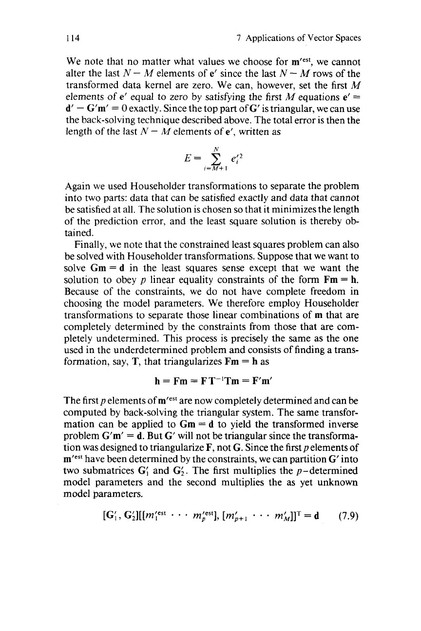
Since the first
p
elements of
mlest
have been determined by the constraints, we can partition
G’
into
two submatrices
G{
and
G;
.
The first multiplies the p-determined
model parameters and the second multiplies the as yet unknown
model parameters.
7.3
Designing Householder Transformations
115
The equation can be rearranged into standard form by subtracting the
part involving the determined model parameters:
(7.10)
The equation is now a completely overdetermined one in the
M
-
p
unknown model parameters and can be solved as described above.
Finally, the solution is transformed back into the original coordinate
system by
mest
=
T-lmlest.
G;[mL+,
* *
-
mh]T=d
-G{[m'est
1
. . .
mFstIT
7.3
Designing Householder
Transformations
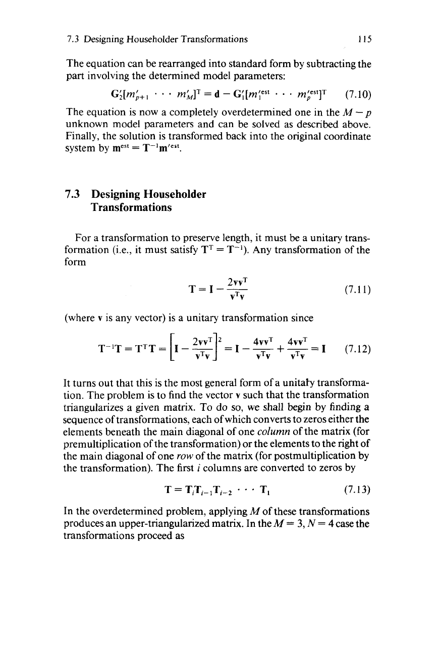
For a transformation to preserve length, it must be a unitary trans-
formation (i.e., it must satisfy
TT
=
T-I).
Any transformation of the
form
(7.1 1)
(where
v
is any vector) is a unitary transformation since
It turns out that this is the most general form of a unitah transforma-
tion. The problem is to find the vector
v
such that the transformation
triangularizes a given matrix.
To
do
so,
we shall begin by finding a
sequence
of
transformations, each
of
which converts to zeros either the
elements beneath the main diagonal of one
column
of the matrix (for
premultiplication of the transformation) or the elements to the right of
the main diagonal of one
row
of the matrix (for postmultiplication by
the transformation). The first
i
columns are converted to zeros by
T
=
TiTi-,Ti-,
-
*
T,
(7.13)
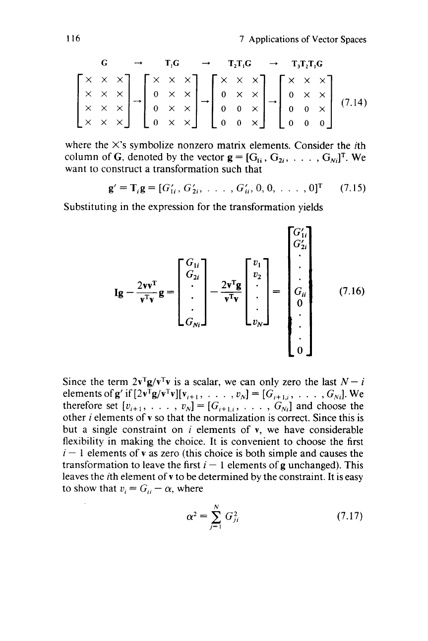
In the overdetermined problem, applying
M
of these transformations
produces an upper-triangularized matrix. In the
M
=
3,
N
=
4
case the
transformations proceed as
116
7
Applications
of
Vector Spaces
xxx xxx xx
[:
xxx
:
:I+[
H
;
;I-[:
00
;
where the
X’s
symbolize nonzero matrix elements. Consider the ith
column of
G,
denoted by the vector
g
=
[GI,,
G2,,
. .
.
,
GJ.
We
want to construct a transformation such that
g’
=
T,g
=
[G;,
,
G;,,
.
.
.
,
G;,,
0,
0,
. . .
,
OIT
(7.15)
Substituting in the expression for the transformation yields
--
VTV
(7.16)
Since the term
2vTg/vTv
is a scalar, we can only zero the last
N-
i
elementsofg’if[2~~g/v~v][v,+~,
.
.
.
,ON]
=
[G,+I,,,
.
.
.
,
GNJ.
We
therefore set
[v,+
,
.
. .
,
UN]
=
[
G,+
,
. .
.
,
GN,]
and choose the
other
i
elements of
v
so
that the normalization is correct. Since this is
but a single constraint on
i
elements of
v,
we have considerable
flexibility in making the choice. It is convenient to choose the first
i
-
1
elements of
v
as zero (this choice is both simple and causes the
transformation to leave the first
i
-
1
elements of
g
unchanged). This
leaves the ith element of
v
to be determined by the constraint. It is easy
to show that
v,
=
G,,
-
a,
where
N
a2
=
G,?,
j=
I
(7.17)
7.4
Transformations That
Do
Not
Preserve Length
117
(Although the sign of
a
is arbitrary, we shall show in Chapter 12 that
one choice is usually better than the other in terms of the numerical
stability of computer algorithms.) The Householder transformation is
then defined by the vector as
v
=
[O,
0,
. . .
>
0,
GI,
-
a,
Gl+i,t, G1+2,r,
.
.
.
>
G,v,IT
(7.18)
Finally, we note that the (i
+
1)st Householder transformation does
not destroy any of the zeros created by the ith, as long as we apply them
in order of decreasing number of zeros. We can thus apply a succession
of these transformations to triangularize an arbitrary matrix. The
inverse transformations are also trivial to construct since they are just
the transforms of the forward transformations.
7.4
Transformations That
Do
Not
Preserve
Length
Suppose we want to solve the linear inverse problem
Gm
=
d
in the
sense of finding a solution
mest
that minimizes a weighted combination
of prediction error and solution simplicity as
(7.19)
It is possible to find transformations
m’
=
T,m
and
e’
=
Tee
which,
although they do not preserve length, nevertheless change it in pre-
cisely such a way that
E
+
L
=
e’Te’
+
m’Tm’
[Ref. 201. The weighting
factors are identity matrices in the new coordinate system.
Consider the weighted measure of length
L
=
mTW,m.
If
we could
factor the weighting matrix into a product of two equal parts, then we
could identify each part with a transformation of coordinates as
L
=
mTW,m
=
mT{TT,T,>m
=
(T,m)T{T,m)
=
m’Tm’
(7.20)
This factorization can be accomplished by forming the eigenvalue
decomposition of a matrix. Let
A,
and
U,
be the matrices
of
eigen-
values and eigenvectors of
W,,
respectively. Then
W,
=
U,A,UL
=
{U,JZ2){AZ2UL}
Minimize
E
+
L
=
eT Wee
+
mT W,m
=
(AZ2UL)T{AZ2UL)
=
TLT,
(7.21)
A
similar transformation can be found for the
W,.
The transformed