Massoud M. Engineering Thermofluids: Thermodynamics, Fluid Mechanics, and Heat Transfer

Подождите немного. Документ загружается.

7. Power Producing Systems, Greenpower Plants 21

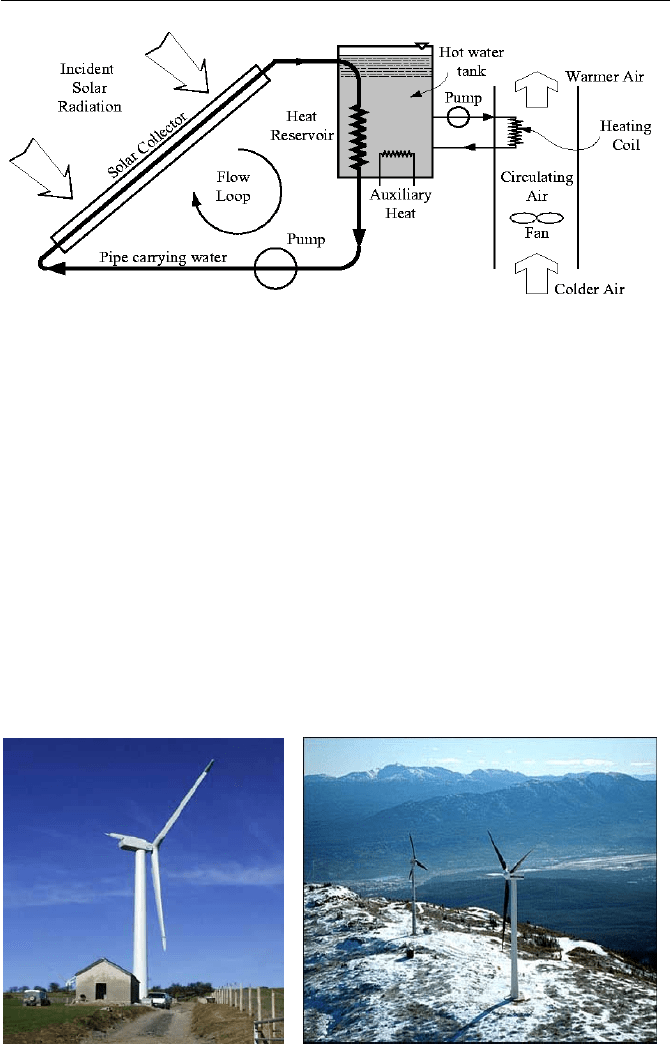
Figure I.7.5. Schematic of space heating by solar energy

7.3. Wind Turbines

Wind turbines convert wind kinetic energy into electricity. The principle of wind

turbines is further discussed in Chapter VIc. Among the various types of wind

turbines, the most popular is the 3-blade horizontal shaft turbine installed on a

tower. The power produced by such turbines is in the range of 0.5 to 1.5 MW.

Due to the low density of air, wind turbines must sweep a wide area to produce

sufficient torque. One of North America’s largest wind turbines produces 1.8 MW

of electricity at 29 rpm. This turbine uses 39 m (128 ft) long blades installed on a

78 m (256 ft) high tower. Examples of three-blade horizontal-shaft wind turbines

are shown in Figure I.7.6. Other types of such turbines include the vertical axis

wind turbine. This machine resembles a giant eggbeater and was patented by

George Darrieus in 1931. The advantage of the Darrieus turbine is that there is no

need for a yaw mechanism to direct the blades towards the wind and the gearbox

is closer to the ground hence, providing easier accessibility.

Figure I.7.6. Horizontal shaft wind turbine

22 I. Introduction

7.4. Tidal Power

Power plants for harnessing tidal power are similar to hydroelectric plants, but are

in the sea instead of in a river beds. The motive power comes from the fact that

the moon’s gravitational effect results in daily high and low tides. The daily surge

of water passes through hydroturbines. The first tidal power plant, generating

over 300 MWe, was built on the Rance River in France to harness the tidal power

of the English channel (Marion). From low to high tide, water rises as much as 44

ft (13.4 m). The plant operates by opening the gates as tide rises to let the channel

water enter the Rance River Dam. The gates are then closed at high tide. The

trapped water is allowed to flow back to the English Channel at low tide through

as many as 24 hydroelectric turbines each producing about 13 MWe. The total

energy from tidal power worldwide is estimated at about 2 GWe

7.5. Geothermal Power

The earth’s core, due to the formation of the solar system some 4.5 billion years

ago, is extremely hot. Indeed at a depth of 40 km, temperature reaches as high as

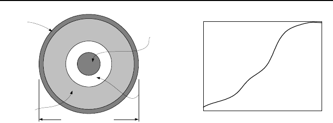
1000 C. Earth’s cross section is shown in Figure I.7.7(a). It is estimated that

7E11 m

of superheated water (as defined in Chapter IIa) at 200 C exists beneath

the earth’s surface (Marion).

Geothermal energy relies on this heat source for power production. In the early

part of the 20

century, the potential of geothermal energy for power was recog-

nized. Larderello, the first geothermal power plant was developed in Italy’s Tus-

cany in 1904. The Larderello plant now produces about 400 MWe. Several other

countries such as Bolivia, Iceland, Japan, New Zealand, and the U.S. use geother-

mal energy for power production. In Reykjavik, Iceland, most houses are heated

with pipes carrying hot volcanic water. In the United States, potential sites for

geothermal energy are found mostly in the Western states such as California, Ne-

vada, and Oregon. Figure I.7.7(b) shows that in 3 decades, power production from

geothermal energy in the U.S. has increased by a factor of about 30. It is esti-

mated that by 2010, power production from geothermal sources in the U.S. will

reach 5–10 GWe. Unlike solar and wind, geothermal energy has a very high de-

gree of availability hence; it is used as base load for power production. Indeed,

the average availability for such plants exceeds 95% compared with about 70% for

coal and 90% for nuclear plants. The negative aspects include a) unlike solar and

wind, geothermal energy is not a 100% renewable source, as long-term use of

such sites would result in steam production at lower pressures or eventual deple-

tion of the source, b) production of such gases as hydrogen sulfide (H

S), carbon

dioxide (CO

), and nitrogen oxide (NO

), albeit these byproduct gases are pro-

duced in a much smaller scale compared to coal power plants, and c) the removal

of underground steam and water can potentially cause the surface to subside. De-

spite these shortcomings, geothermal energy is indeed a very useful and clean

source of energy, and with improving economical aspects it is expected to meet an

increasing share of the world’s energy needs.

8. Comparison of Various Energy Sources 23

Crust

Mantle,

Magma

& Rock

Magma

Iron Core

8,000 miles

1970

1980 1990 2000

3000

2000

1000

Power (MWe)

Year

(a) (b)

Figure I.7.7. Depiction of: (a) Earth’s cross-section; (b) growth of geothermal power in the

U.S.

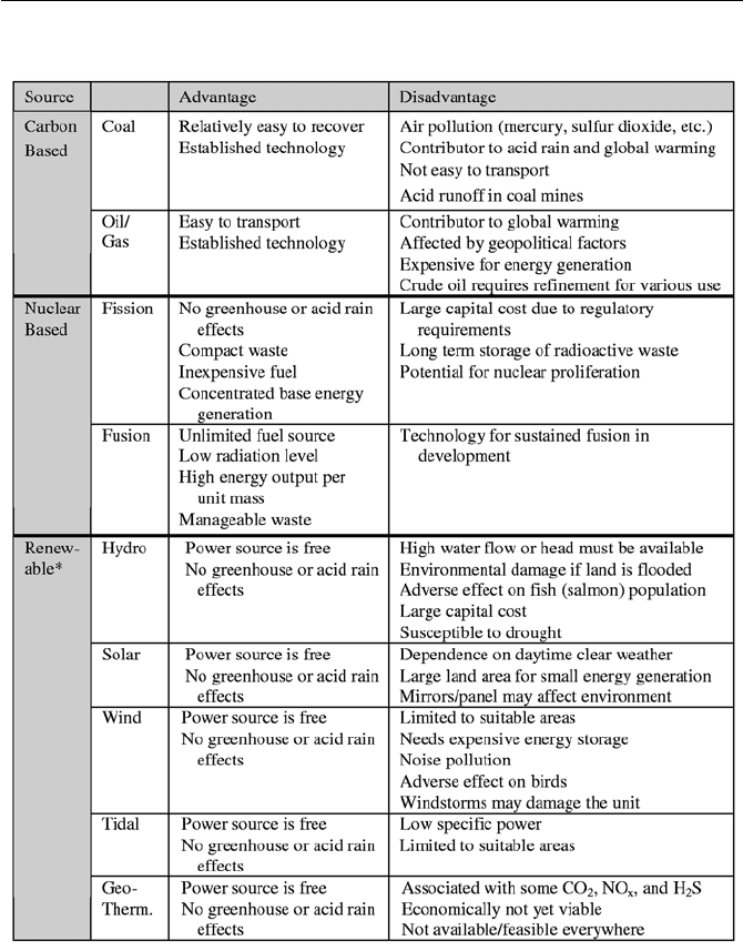
8. Comparison of Various Energy Sources

In Table I.8.1, we have divided the various sources of energy into three major

categories as follows.

Carbon-based fuels. While this type of fuel has been the major source of en-

ergy for the past two centuries, it is coming under increasing scrutiny. This is be-

cause byproducts of carbon-based fuels include CO

as well as other gases, re-

ferred to as the greenhouse gases. Greenhouse gases in the upper atmosphere trap

the sun’s radiation and increase the retention of thermal energy, which otherwise

would have been reflected back into space. Hence, these gases result in an in-

crease in the earth’s temperature. This phenomenon, known as the greenhouse ef-

fect is thought to be responsible for global warming.

Nuclear fuels. Nuclear-based energy is combustion free and there are therefore

no emissions. However the operational safety and the safe disposal of nuclear

waste remain a matter of public concern. The nuclear industry has made substan-

tial improvement in operational safety. The new generation of reactors is designed

to maximize safety and reliability by enhancing the passive safety features and re-

ducing reliance on pumps, valves, and emergency diesel generators. Regarding

nuclear waste disposal, nuclear plants store the spent fuel assemblies on-site in

spent fuel pools, which in many plants have reached their maximum capacity.

Nuclear plants in the U.S. have then started to store the oldest spent fuel assem-

blies in dry storage canisters, which are then housed on-site for passive cooling for

eventual transfer to the federal repository at Yucca Mountain, Nevada.

Greenpower. The major problem associated with the renewable resources is

low power density, defined as power produced per site area (MW/m

24 I. Introduction

Table I.8.1. Comparison of various sources of energy

* Not shown in this table is the biomass energy source. Biomass includes the organic ma-

terial, which convert the sunlight energy into chemical energy, which is then converted

to heat when burned. Biomass fuels include such materials as wood, straw, ethanol,

manure, sugar cane, and other byproducts from a variety of agricultural processes.

9. Thermofluid Analysis of Systems 25

As Table I.8.1 shows, much research and development are needed to find an

optimum solution to the issue of energy production. This is because on the one

hand with an increasing world population and with energy being a major contribu-

tor in the advancement of society, one can expect that energy consumption would

have only an upward trend. On the other hand, the environmental impacts associ-

ated with various sources of energy are testing the tolerance level of our planet.

Regarding the greenhouse effect, while, the impact of CO

production on the

global atmosphere is still a topic of debate and investigation, it is reasonable to

conclude that the production of such gases should be limited. This would in turn

limit the use of carbon-based fuels. We then face the problem of finding a suitable

substitution to make up for the partial loss of power production from carbon-based

energy sources. Our choice for this purpose is indeed limited, given the associated

disadvantages of other sources of energy. Since fusion technology is seemingly

remote, the two long term alternatives at the present time seem to be the fission

reactors with enhanced safety features and geothermal power.

8.1. Saving Energy by Enhancing Efficiencies

An important factor in meeting the energy demand is the application of technology

in increasing efficiency at the three stages of production, transmission, and con-

sumption. The electricity produced in most central power plants using steam tur-

bines, is about 1/3 of the total energy consumed. The remaining 2/3 is wasted as

rejected heat to the environment. The central stations using gas turbines may have

efficiencies in excess of 45% mostly due to operation at higher gas temperatures

compared with steam temperature. Voltage drop in transmission lines has been a

topic of investigation to find materials, which pose less resistance to the flow of

electricity. Superconducting materials have such ability but they must presently

operate at very low temperatures. Finally, improvement of efficiency in such

home appliances as refrigerators, hot water heaters, heat pumps, washers and dry-

ers would help reduce demand for power.

9. Thermofluid Analysis of Systems

Design and operation of any power producing system must satisfy the imposed

constraints such as cost, safety, performance, size, and environmental impact.

Here we focus only on the thermofluid aspects. In Section 4 we introduced such

systems as pump, turbine, reactor vessel, steam generator, condenser, internal

combustion engine, nuclear power plant, wind turbine, etc. There are five funda-

mental equations for the analysis of all such systems. These five fundamental

equations in thermofluid analysis are:

• conservation equation of mass,

• conservation equation of energy,

• conservation equation of momentum (also known as linear momentum),

26 I. Introduction

• conservation equation of angular momentum,

• the second law of thermodynamic

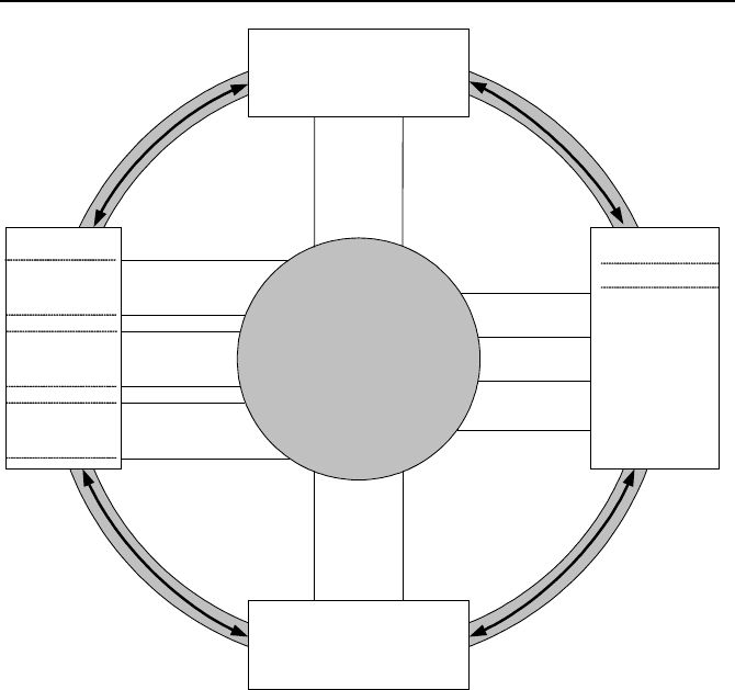
These equations are shown in the hub of Figure I.9.1. However, before these equa-

tions are applied, we first need to determine what we mean by thermofluid analysis

of a system. This in turn requires us to identify the variables that we call design pa-

rameters of a system.

We can divide the design parameters into several categories. For example, one

category includes the system dimensions such as diameter, height, flow area, and

volume. Another category deals with the thermodynamic aspects such as pressure,

temperature, and density. A third category might include parameters related to hy-

drodynamics such as power, momentum, torque, force, acceleration, and velocity.

In any system analysis, some of the design parameters are given and we need to

find some other parameters of interest. This is what we refer to as thermofluid

analysis of a system.

To perform thermofluid analysis of a system, we must first determine the extent

of the system. This is accomplished by using techniques known as control volume

and control mass as described in Chapter IIa. Once the extent of the system is de-

fined, we consider the process applied to the system to identify the appropriate set of

equations to use.

Having determined the systen, the involved process, and the specified set of input

data, we must then ensure that the number of applicable fundamental equations is

sufficient to uniquely determine the number of the design parameters, which are un-

known. Also not all the five fundamental equations listed above are applicable to

the analysis of a system. For example, if there is no rotational motion involved in

the analysis, the conservation equation of angular momentum is not applicable.

Even when all the five fundamental equations are applicable, still we may run into

the problem of having more unknowns than equations. This problem is remedied

(i.e., the number of equations are increased to become equal to the number of un-

knowns) by introducing additional equations known as the constitutive equations,

shown as spokes in Figure I.9.1. This figure is one way to visualize the interrelation

between the fundamental and the constitutive equations.

Application of the constitutive equations depends on the type of analysis. If the

analysis involves heat transfer, temperature and the rate of heat transfer are related

by a constitutive equation. This constitutive equation, as discussed in Chapter IV,

depends on the mode of heat transfer involved in the process. For example, in con-

duction heat transfer, the related constitutive equation is known as Fourier’s law of

conduction. Similarly, in convection heat transfer, the related constitutive equation

is known as Newton’s law of cooling while, in radiation heat transfer, the related

constitutive equation is known as the Stefan-Boltzmann law.

The constitutive equations in fluid mechanics, as discussed in Chapter III, are

primarily the Newton’s law of viscosity and the Stokes hypothesis. The constitutive

equation in mass transfer is the Fick’s law of diffusion. The set of constitutive equa-

tions that is most often used is the equation of state relating the thermodynamic

variables of a system. These thermodynamic variables are known as properties, as

discussed in Chapter IIa.

9. Thermofluid Analysis of Systems 27

Newton's Law

of Cooling

Stefan-Botlzmann

Law

Stokes

hypothesis

Newton's Law

of Viscosity

Fick's Law

Conservation of Mass

Conservation of Momentum

Conservation of Angular Momentum

Conservation of Energy

Second Law of Thermodynamics

Thermodynamics

Mass Transfer

Heat Transfer

Conduction

Convection

Radiation

Fluid Mechanics

Hydro Static

Hydro

Dynamic

Equation

of State

Volume

Constraint

of Conduction

Fourier's Law

Figure I.9.1. Possible classification of the fundamental (Hub) and the constitutive (Spoke)

equations in thermofluid analysis of systems

QUESTIONS

− What types of energy conversion take place in shoveling snow, rowing a canoe,

and riding the elevator?

− What is the role of a transformer in the transmission of electricity through the

power lines?

− How do you classify condensers, automotive radiators, and cooling towers?

− Is it true to say that the energy associated with fission is primarily due to the re-

leased radiation?

− What is the difference between fission and fusion?

− Are fossil power plants using coal for fuel, considered external or internal com-

bustion machines?

− Why does the diameter of a steam turbine rotor increase as steam pressure de-

creases?

− Why is a nuclear reactor especially well suited for submarines?

28 I. Introduction

− How does a gas turbine operate?

− What are the differences between turbofan, turboprop, and turboshaft?

− What is the key factor in favor of jet engines over internal combustion engines

for aviation application?

− Name a disadvantage associated with hydropower plants?

− What are the disadvantages associated with wind power?

− What are the conservation equations? What do they conserve? Is the equation

formulating the second law of thermodynamic a conservation equation?

− What is a constitutive equation? Why do we often need to use a constitutive

equation?

PROBLEMS

1. Match the upper case with the lower case letters that best describe the conver-

sion of energy:

A. chemical – electrical, B. solar – electrical, C. electrical – thermal, D. nuclear –

thermal, E. electrical – mechanical, F. chemical – mechanical, G. kinetic – ther-

mal, H. potential – kinetic.

a. free fall, b. battery, c. plane crash, d. motor, e. solar calculator, f. heater, g. nu-

clear power plant, h. body muscles.

2. Use your knowledge of power production, power consumption, and energy con-

version to find the names of the systems shown as a and b in the left hand and c

and d in the right hand schematics. [Ans.: a is a hydraulic turbine].

Head

Water

Tail

Water

Electric Power

Tail

Water

Head Water

3. Explain the role of energy in water desalination and draw a diagram to represent

the operation of such plant. First consider the goal and then try to find the means

to accomplish your goal.

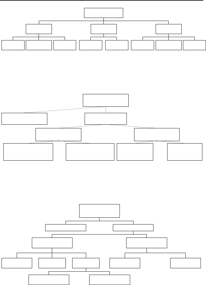
4. A simplified diagram of the three major energy sources and examples of each

source of energy are shown below. Provide additional examples for sources of en-

ergy known as renewable sources or greenpower, and provide a brief description

for each of the examples.

Questions and Problems 29

Sources of Energy

Fossil Nuclear Greenpower

Coal Oil Gas Hydro Wind SolarFission Fusion

5. Principles of electrical energy production are shown in the simplified diagram.

Provide a brief summary for each box comprising the thermodynamic cycle.

Electric Power

Production

Thermodynamic

Cycle

No Thermodynamic

Cycle

Internal

Combustion Machines

External Combustion

Machines

Hydropower Wind & Tidal

Direct Energy

Conversion*

Faraday's Law

of Induction

* Some direct energy conversion systems such as magnetohydrodynamics use the Faraday law of induction

6. A simplified diagram for nuclear power is shown below. Provide a brief de-

scription for each box comprising the light water reactor type.

Nuclear Power

FissionFusion

Thermal Reactor Fast Reactor

Heavey Water

(CANDU)

Light Water Gas Coolded Liquid Metal

Pressurized Water Boiling Water

Gas Coolded

7. A gas-cooled reactor uses a compressor to circulate helium as the working fluid,

through the core of the reactor. The heated gas then enters a gas turbine to pro-

duce power. Helium is then cooled in the condenser and pumped back to the reac-

tor. Another gas cooled plant uses a similar cycle but hot gases instead of entering

a gas turbine enter a steam generator to boil water in the secondary side. The

30 I. Introduction

cooler gas enters the compressor to be pumped back into the reactor and steam in

the secondary side of the steam generator enters a steam turbine. Draw the flow

path of the working fluid in each reactor type and describe the advantages and dis-

advantages of each design.

8. Use schematic diagrams to draw the flow path of both a BWR and a PWR. Ex-

plain the flow path in the reactor core for both types of reactors and the flow path

in the steam generator of the PWR.

9. During normal operation of a PWR, feedwater enters the secondary side of the

steam generator. After being heated by the hotter primary side water, feedwater

boils in the tube bundle and dry steam leaves the steam generator and flows to-

wards the turbine through the main steam line. In this condition, water level in the

steam generator remains at a fixed level. Is it fair to say that the flow rate of steam

out of the steam generator exactly matches the flow rate of the feedwater into the

steam generator?

10. Describe the operation of a thermodynamic cycle. List and discuss the role of

the various components of a thermodynamic cycle. Describe the operation of a

Wankel engine in the framework of a thermodynamic cycle. In this regard, iden-

tify the heat source, the heat sink, and the working fluid in an internal combustion

engine such as a Wankel rotary engine.