Massoud M. Engineering Thermofluids: Thermodynamics, Fluid Mechanics, and Heat Transfer

Подождите немного. Документ загружается.

392 IIIb. Fluid Mechanics: Incompressible Viscous Flow

Pipe LD K

No. (ft) (in) (-)

1 100.00 5.00 50.00

2 80.00 4.50 45.00

3 70.00 4.00 65.00

4 120.00 3.50 55.00

5 90.00 3.00 15.00

[Ans.:

Flow In Serial Pipes

Pipe

No.

(ft)

(in)

(ft

)

(ft/s)

(-)



GPM

× 1E–6

(-)

∆P

(psi)

1 100 5.00 0.136 3.27 50.00 200 0.121 0.0177

3.90

2 80 4.50 0.110 4.05 45.00 200 0.135 0.0173

5.33

3 70 4.00 0.087 5.12 65.00 200 0.152 0.0169

12.03

4 120 3.50 0.067 6.65 55.00 200 0.173 0.0164

18.49

5 90 3.00 0.049 9.09 15.00 200 0.202 0.0159

11.51

Data For The Equivalent Pipe Representing The Compound Piping System

L (ft) D (in) A (ft

) V (ft/s) K(-) V



(GPM) I (ft

-1

)

∆P(psi)

491.48 3.06 0.083 5.37 233.02 200.00 5159.06 51.3].

50. Water flows at a rate of 5000 GPM into a piping system connected in parallel.

Length, diameter, and loss coefficient of each branch are given below. For

62.4 lbm/ft

and v = 9.305E-6 ft

/s find total pressure drop and the length and di-

ameter of an equivalent pipe representing this system.

Pipe L D K

No. (ft) (in) (-)

1 1000.0 10.00 150.00

2 1500.0 11.00 100.00

3 500.00 8.00 10.00

4 2000.0 9.00 50.00

5 900.00 7.00 5.00

[Ans.:

Flow In Parallel Pipes

Pipe

No.

(ft)

(in)

(ft

)

(ft/s)

(-)



GPM

× 1E–6

(-)

∆P

(psi)

1 1000 10.00 0.545 5.20 150.00 1272.69 0.47 0.01353 3.39

2 1500 11.00 0.660 4.61 100.00 1365.92 0.45 0.01359 3.39

3 500 8.00 0.349 7.04 10.00 1102.76 0.50 0.01331 3.39

4 2000 9.50 0.442 3.51 50.00 696.99 0.28 0.01494 3.39

5 900 7.00 0.267 4.68 5.00 561.64 0.29 0.01484 3.39

Questions and Problems 393

Date of the Equivalent Pipe Representing the Compound Piping System

L (ft) D (in) A (ft

) V (ft/s) K(-) V



(GPM) I (ft

-1

) ∆P(psi)

1154.48 10.51 2.263 4.922 31.56 5000 510.05 3.39].

Section 5

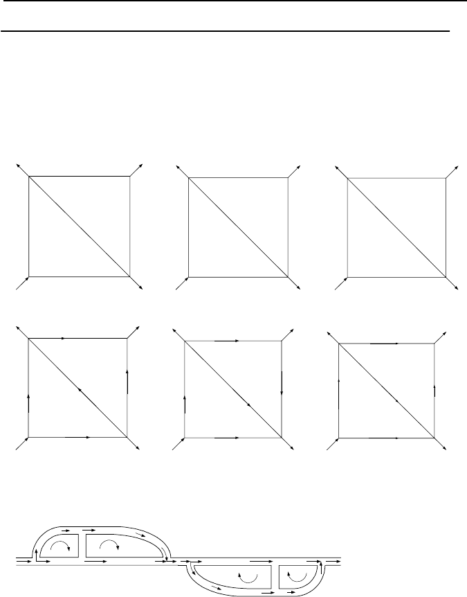
51. Find flow distribution in each network by the Hardy Cross method. Assume n

= 2. Try the same cases for n = 1.8.

c = 8

c = 5

c = 15

c =10

c = 4

c = 3

c = 2

c =1

c = 5

c = 3

c = 15

c = 7

[Ans.:

3.326

53.907

11.737

46.093

11.174

53.774

1.174

46.226

87.249

169.150

80.350

62.751

52. Find the absolute value of the flow rate and the direction of the flow in

branches BC and FG.

1.5 m

IVIII

Pipe 1 2 3 4 5 6 7 8 9 10

L (m) 585 253.8 223.2 9.77 18.1 1269 565.3 201.3 19.6 6.8

D (m) 0.65 0.55 0.45 0.35 0.30 0.55 0.50 0.40 0.35 0.30

[Ans.: 0.0 and 0.007 m

/s from G to F].

53. Write a computer program based on the Hardy Cross method for determina-

tion of flow distribution in piping networks. First, start with simple cases and use

the methods outlined in Chapter IIIb.5 before extending to more general cases.

394 IIIb. Fluid Mechanics: Incompressible Viscous Flow

Section 6

54. Derive the time to drain the tank of Example IIIb.6.2 from the observation

that t = V

. [Hint: Use an average value for V

= 2/h2

g and the fact that

= h

55. An emergency water tank is pressurized with nitrogen to 1.0 MPa. The tank

has a diameter of 2 m. Height of water in the tank is 15 m. The tank is located

above a reactor and is connected to the reactor by a pipe having a diameter of 0.2

m. At time zero the reactor pressure drops to 0.2 MPa. Find the maximum flow

rate delivered by the tank to the reactor. Treat water as an ideal fluid (incom-

pressible and inviscid). [Ans.: 1367 kg/s].

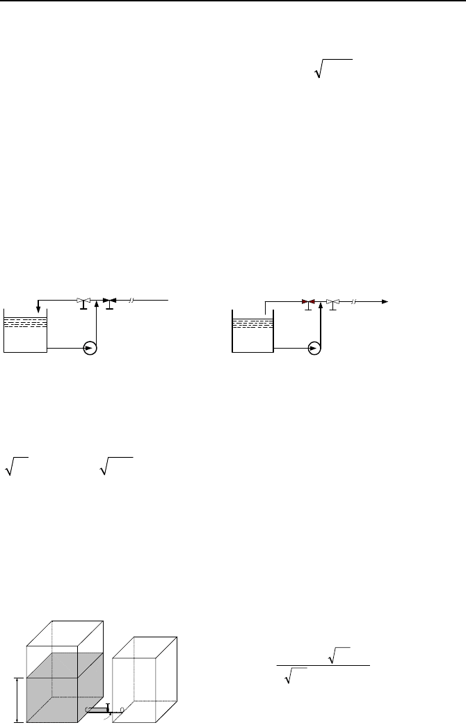
56. A pump is operating in recirculation mode. At time zero, we close the bypass

valve and simultaneously open the isolation valve to fill the initially drained sup-

ply line. Use the data to find the time it takes to fill the supply line. Data:

V200

pump



GPM, L

Supply Line

= 1200 ft, D

Supply Line

= 3 in. [Ans.: ~ 132 s].

Isolation

Valve

Bypass

Valve

Isolation

Valve

Bypass

Valve

57. A water tank, in the shape of a right circular cylinder, has an inside diameter

D. The tank, being open to the atmosphere is initially filled with water up to a

height of h

, measured from the drain centerline. The drain has an inside diameter

d and a discharge coefficient of C

. We now open the drain to drain the tank by

gravity. Show that the time to drain the tank is obtained from t =

h/[ (/ ) /2]

CdD g

58. A water tank is at atmospheric pressure. Initially, the tank water level is at 20

ft from the drain centerline. We now open the drain and assume there are no fric-

tional losses. If A

= 0.015, find the time to drain the tank.

59. Consider two rectangular tanks having constant flow areas of A

and A

. The

tanks are connected at the bottom by a frictionless pipe of diameter d. The first

tank is filled with water up to an elevation h

from the connecting pipe. We now

open the isolation valve. a) Show that the time for levels to equalize is given by:

d, a

CAAga

)(2

Questions and Problems 395

b) Find the time in second if h

= 3 m, d = 5 cm, A

= 3 m

, A

= 2 m

, and C

0.61. [Ans. 7 m, 21 s].

60. The initially closed valve in Figure IIIb.6.1(b) suddenly opens. Find the time

it takes velocity to reach 99% of its steady-state value. Assume that fluid is invis-

cid and L = 30 ft, h

= 7 ft, D = 1 in. [Ans.: 7.5 s].

61. The initially closed valve in Figure IIIb.6.1(b) suddenly opens. Find the flow

velocity 5 seconds after the valve is opened. Data: L = 1000 ft, h

= 50 ft, V

= 10

ft/s. [Ans.:

λ = 3.1 s. and V = 6.7 ft/s].

62. A tank in the shape of a right circular cylinder (Figure IIIb.6.3.) contains wa-

ter and is pressurized to 50 psia. Water level from the drain centerline is 15 ft.

The tank height is 20 ft, tank diameter is 10 ft and the drain diameter is 1 in. Find

the time to completely drain the tank. The water tank is fully insulated. Do you

expect some water flashing to steam when level becomes near zero? What hap-

pens if we use an exceedingly small hole for the drain? [Ans.: 200 min]

63. A capillary tube viscometer, as shown in the figure, is a reservoir containing

oil, connected to a capillary tube (d on the order of 1 mm). Find the time to drain

oil from the reservoir.

Oil

reservoir

Capillary

tube

[Ans.:

1ln)(

64. Oil (v = 1E–4 m

/s), enters an open tank at a steady rate of 2 m

/min and

leaves through a 25 m long pipe. The Tank has a constant cross sectional area of 3

and the pipe has an inside diameter of 15 cm. At steady state conditions, the

exit pressure is 2 m of oil. While the inlet flow remains constant, we increase the

exit pressure instantaneously to 3 m of oil. Find the effect on oil level and exit

flow rate.

65. Oil (v = 1E–4 m

/s), enters an open tank at a steady rate of 2 m

/min and

leaves through a 25 m long pipe. The Tank has a constant cross sectional area of 3

and the pipe has an inside diameter of 15 cm. At steady state conditions, the

exit pressure is 2 m of oil. While the inlet flow remains constant, we increase the

exit pressure linearly to 4 m of oil in 5 minutes. Find the tank oil level at 5 min-

utes, i.e., when h

= 4 meters.

66. A gas tank of volume V contains pressurized gas at pressure P

and tempera-

ture T. Flow rate of gas into and out of the tank under steady-state conditions is



. Pressure at point C, Figure IIIb.6.10(a), jumps to: P

= P

+ ∆P. Find the

396 IIIb. Fluid Mechanics: Incompressible Viscous Flow

tank pressure versus time. Tank is not insulated hence process is isothermal. As-

sume laminar flow in the discharge pipe.

[Ans.: )()()(

)/KV/(

1 CCoo

RTt

CCo

PPPePPtP −−+−=

−

67. A tank having a volume of 30 m

contains air at 400 kPa. We intend to

charge this tank through a feed line having a diameter of 4 cm and a length of 30

m. Pressurized air at 900 kPa and 15 C enters the feed line. Find the time it takes

for the tank pressure to reach 900 kPa.

68. A tank having a volume of 40 m

contains air at 500 kPa. We intend to

charge this tank through a feed line having a diameter of 4 cm and a length of 30

m. Pressurized air at 900 kPa and 15 C enters the feed line. Find the tank pres-

sure after 2 minutes. Plot the tank pressure and the inlet mass flow rate versus

time.

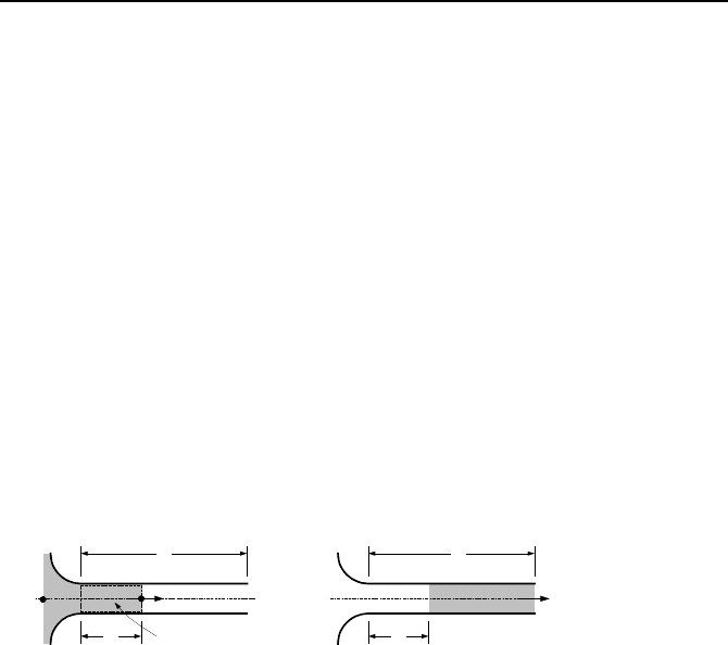
69. Consider two identical pipes. One pipe is to be filled with water by suddenly

raising the liquid pressure upstream of the pipe to P

. The other pipe is already

filled with water. We would like to expel the water from the pipe by suddenly in-

creasing the upstream pressure of the gas to P

. Find the time to fill and to drain

each pipe and compare the results. The atmospheric pressure for both cases is

shown by P

. Pipe area is A.

L L

Control Volume

[Hint: For the filling the pipe example, write the momentum equation for the

control volume shown in the figure as

ΣF = d(mV)/dt + ∆(momentum flux). Since

no mass is leaving, momentum flux at the exit is zero and momentum flux at the

inlet is the flow rate into the control volume. The momentum equation then be-

comes:

– P

)A – F

friction

= d(mV/dt) + (0 –



Relate



to m from the continuity equation and substitute for m from

Ax and

for V from V = dx/dt].

70. Shown in the figure is a normally closed control valve known as the contain-

ment spray isolation valve, being generally a motor operated globe valve. In case

of a hypothetical accident that leads to containment pressurization, a spray signal

is sent to turn on the pump and open the control valve. The piping upstream of the

spray valve is filled with water whereas the piping downstream of the control

valve is drained. When the signal is sent to activate the spray system, the control

valve begins to open, water starts to flow in the empty piping until it eventually

reaches the spray header located at an elevation of about 200 ft. Water is then

sprayed into the containment atmosphere at a desired droplet diameter by 100

spray nozzles attached to the header ring. You are to determine the time it takes to

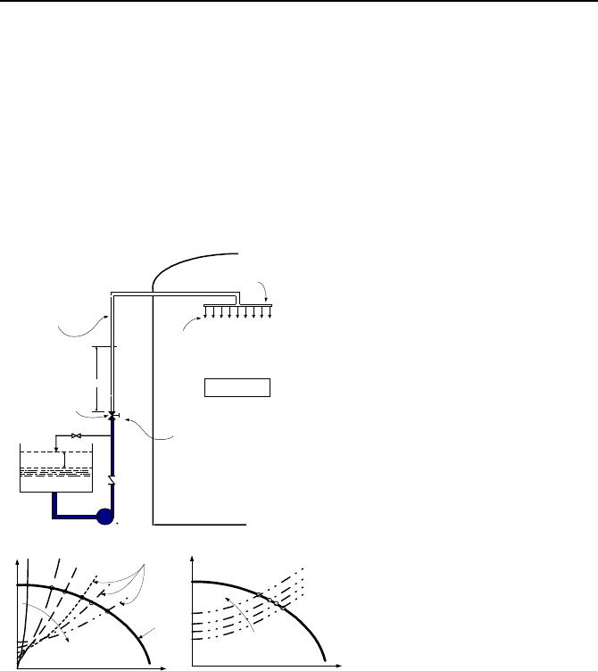
Questions and Problems 397

fill the pipeline and to calculate the flow rate out of the nozzles once the header is

filled.

[Hint: This can be calculated by dividing the volume of the drained pipe by the

volumetric flow rate. Since, flow rate is changing with time this should be done in

a discretized manner. To simplify the analysis, you may assume that the pump is

operating at rated conditions and flow is bypassed to the reservoir. Then a signal

is sent to the control valve to open. This signal simultaneously closes the bypass

valve. The first plot shows the system curve when the control valve is opening

and the second plot shows the system curve when the control valve is fully

opened].

h=f

(t)

y=f

(t)

m=f

(t)

1: Water surface in reservoir

X: Water level at time t

2: Containment atmosphere

Drained Pipline to

be Filled With Water

Control Valve

Spray Header

Spray Nozzle

Containment

Bypass Valve

Spray Pump

System

Curves

Pump

Curve

Z = f(t)

71. A spherical bubble of nitrogen, having an initial diameter of 5 mm is released

at a depth of 10 m in a pool of water. Assume the bubble instantly reaches its

terminal velocity. Find the time it takes for the bubble to reach the water surface.

Plot d, V, and h as a function of time and comment on the validity of the results.

72. A pipe equipped with a nozzle is used to deliver water to the wheel of a hy-

draulic turbine. The pipe has a diameter of 35 cm and a length of 1 km. The noz-

zle has a diameter of 10 cm and provides a velocity head of 35 m when turbine

operates at steady state condition. Now, consider a case where the fully closed

turbine stop valve is suddenly opened. Find the time it takes the wheel of the tur-

bine to reach 97% of its full speed.

398 IIIb. Fluid Mechanics: Incompressible Viscous Flow

Section 7

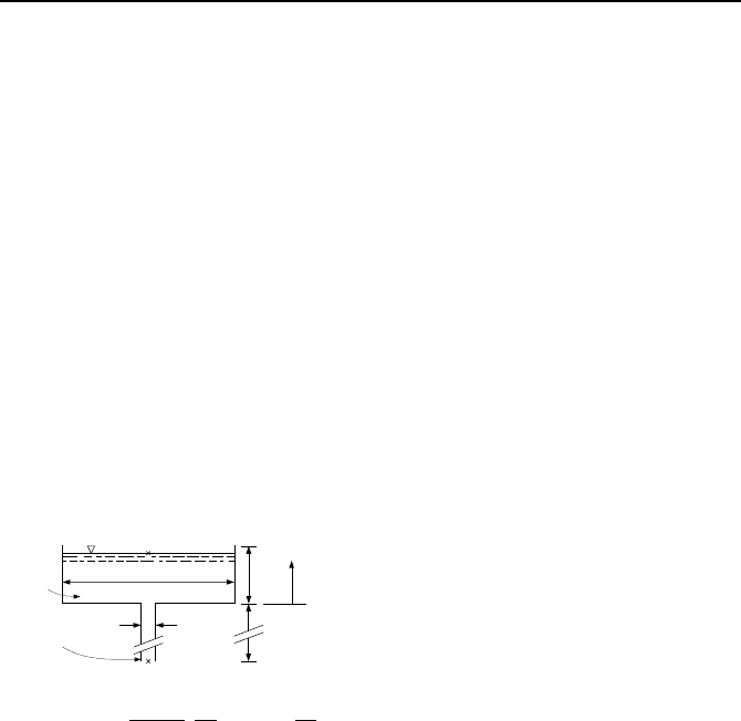
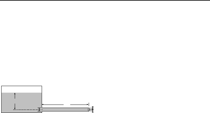
73. A large tank is connected to a pipe of diameter D and length L. Water is

flowing steadily in the pipe, which is discharged to the atmosphere. A blanket of

gas is used to maintain pressure in the tank at P

= P

. At time zero, we increase

the gas pressure so that P

(t) = f(t). Use the assumptions consistent with the rigid

column theory and find the governing differential equation for the flow rate in the

pipe. Plot flow rate versus time for the following data. By adding water, the tank

water level is constantly maintained at H. Data: P

= 20 psia, H = 10 ft, L = 1 ft,

D = 1 in, f(t) = (2P

/5)t + P

for t ≤ 5 s and f(t) = 3P

for t > 5 s. Assume smooth

pipe.

74. Water flows at 60 F in a 12-inch Schedule 40 pipe (D = 11.938 in. and

0.406 in.). Find the head rise due to the instantaneous closure of a valve a) for

steel pipe and b) for a PVC pipe having the same dimensions as the steel pipe.

water

= 62.37 lbm/ft

, (E

)

water

= 3.11E5 psi. V



= 2442 GPM.

75. Consider flow of water in a frictionless pipe at 7 ft/s. An isolation valve is in-

stantaneously closed. Find the resulting pressure head just upstream of the valve.

[Ans.: 4890 × 7/32.2 = 1,063 ft]

76. Water at 60 F is flowing in an 18-inch Schedule 80 steel pipe. Find the wave

speed for the system.

water

= 62.37 lbm/ft

, (E

)

water

= 3.11 × 10

psi.

1. Steady Internal Compressible Viscous Flow

399

III

. Compressible Flow

1. Steady Internal Compressible Viscous Flow

In compressible fluids, changes in the fluid density due to the variation in pressure

and temperature may become significant and the treatment of the flow discussed

in the previous sections should be applied here with added vigilance. Due to the

complexity of the subject, flow of compressible fluids is generally divided into

three categories. These include, flow of gas, flow of two-phase mixture (such as

steam and water), and two-phase flow mixed with non-condensable gases. The

flow path may include a pipe, a Bernoulli obstruction meter (nozzle, thin-plate ori-

fice, and venturi), valves, fittings, and pipe breaks. Compressible fluids may en-

counter a phenomenon known as choked or critical flow. This phenomenon im-

poses an added constraint on the internal flow of compressible fluids and must be

considered in all of the above categories. Failure to do so results in gross errors in

the related analysis.

In this section, we study only the flow of gases in pipes, Bernoulli obstruction

meters, and pipe breaks. In all these cases, the compressible fluid is considered to

behave as an ideal gas undergoing such processes as isothermal, adiabatic, or isen-

tropic. In general, flow of gases in pipelines is associated with heat transfer and

friction. We therefore begin the analysis of steady, one-dimensional, internal flow

of compressible fluids in a variable area conduit with friction and heat transfer.

We then reduce the general formula to obtain the formulation for some specific

processes such as isothermal and adiabatic.

1.1. Compressible Viscous Flow in Conduits

To derive the general formula for one-dimensional flow of ideal gases with fric-

tion and heat transfer, we consider the one-dimensional flow of a compressible

fluid in the variable area conduit of Figure IIIc.1.1. At any location x from the en-

trance to the conduit, the flow field is defined by four parameters P(x), T(x), V(x),

and

(x). To determine these parameters, we use continuity, energy, and momen-

tum equations as well as the equation of state written for differential control vol-

ume A(x)dx. Using the mass, momentum, and energy at steady state conditions

entering the control volume at x, we find the mass, momentum and energy at x

+dx by Taylor’s series expansion. The continuity equation becomes d(

VA) = 0.

The energy equation for steady state, no shaft work, negligible changes in poten-

tial energy, and no internal heat generation becomes

dq = c

dT + VdV IIIc.1.1

where the first term on the right side represents the change in enthalpy from x to

x + dx. The net momentum flux at steady state is equal to the summation of forces

act

ing on the control volume:

VdVDdxdP

ρτ

=−− )/(4 IIIc.1.2

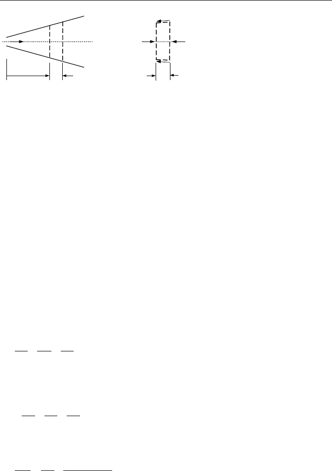
IIIc. Fluid Mechanics: Compressible Flow

400

P + dP

Figure IIIc.1.1. Flow of ideal gas in a variable area conduit with heat transfer and friction

To simplify the momentum equation, we define:

dF = (4/

)(dx/D)

IIIc.1.3

where dF is the frictional head loss per unit mass. Substituting for

from Equa-

tion IIIc.1.3 into Equation IIIc.1.2, we obtain;

– dP –

dF =

VdV IIIc.1.4

The last equation to use is the equation of state for an ideal gas:

d(P/R

T) = 0 IIIc.1.5

The formulation of the problem ends here. To find the four parameters P, T, V

and

, we solve these four equations simultaneously. First, we carry out the dif-

ferentials in the continuity equation and in the equation of state. We then divide

the result by the argument. For example, for the continuity equation we have:

0)( =++= dAVAdVVAdVAd

ρρρρ

IIIc.1.6

Dividing by

VA, we obtain:

0=++

dVd

IIIc.1.7

Similarly, differentiating the equation of state and dividing through by P = R

yields:

0=++−

dTd

IIIc.1.8

For the energy equation, we divide Equation IIIc.1.1 by c

(1)

dq dT V dV

cT T V RT

−

IIIc.1.9

and for the momentum equation, we divide Equation IIIc.1.4 by P:

1. Steady Internal Compressible Viscous Flow

401

γρ

=−− IIIc.1.10

Note that in the energy and momentum equations we also made use of c

(

γ−

1) where

= c

. We now manipulate the definition of the Mach number Ma

= V/c by substituting for the speed of sound in the medium c

RT to obtain Ma

= V

RT). Taking the derivative and dividing by the argument yields:

TdTVTdVd

−=−=

−

)/(

222

IIIc.1.11

which simplifies to:

)

(

dTd

Substituting for dV/V in the energy and momentum equations, we obtain a system

of four algebraic equations for four unknowns dP, dT, dV, and d

. Solving by the

method of elimination and substitution, yields:

22 2

Ma Ma ( 1)Ma 1

1Ma 1Ma 1Ma

dP dq dA dF

cT A RT

γγγ

§·

−−+

§· § ·

=+−

¨¸

¨¸ ¨ ¸

¨¸

−− −

©¹ © ¹

©¹

IIIc.1.12

22 2

222

1Ma (-1)Ma (1)Ma

1Ma 1Ma 1Ma

dT dq dA dF

TcT A RT

γγ γ

§·

−−

§· § ·

=+−

¨¸

¨¸ ¨ ¸

¨¸

−−−

©¹ © ¹

©¹

IIIc.1.13

222

111

1Ma 1M 1Ma

dV dq dA dF

VcTaA RT

§·

§· § ·

=++

¨¸

¨¸ ¨ ¸

¨¸

−−−

©¹ © ¹

©¹

IIIc.1.14

222

1Ma1

1Ma 1Ma 1Ma

ddqdAdF

cT A RT

§·

§· § ·

=+−

¨¸

¨¸ ¨ ¸

¨¸

−−−

©¹ © ¹

©¹

IIIc.1.15

where in these equations, q, A, and F are known functions. Upon the integration

of Equations IIIc.1.12 through IIIc.1.15, we find pressure P, temperature T, veloc-

ity V, and fluid density

, respectively. Next, we derive analytical solutions for

the three important processes: isothermal, adiabatic, and isentropic.

1.2. Isothermal Process For Compressible Flow

To analyze the flow of compressible fluids in an isothermal process, we may use

the general formula obtained above and apply the isotherm constraint or derive the

formulation directly. Both methods are described here.